Figure 1
UMAP on 7 MOFA factors
## UMAP
plot.umap.data <-  plot_dimred(mofa, method="UMAP", color_by = "condition",stroke = 0.001, dot_size =1, alpha = 0.2, return_data = T)

plot.umap.all <- ggplot(plot.umap.data, aes(x=x, y = y, fill = color_by))+
  geom_point(size = 0.8, alpha = 0.6, shape = 21, stroke = 0) +
  theme_half_open() +
  scale_fill_manual(values = colorgradient6_manual, labels = c(labels), name = "Time aIg",)+
   theme(legend.position="none")+
  scale_x_reverse()+
  scale_y_reverse()+
  add.textsize +
  labs(title = "UMAP on MOFA+ factors shows minute and \nhour timescale signal transductions", x = "UMAP 1", y = "UMAP 2")

## UMAP legend
legend.umap <- get_legend( ggplot(plot.umap.data, aes(x=x, y = y, fill = color_by))+
  geom_point(size = 2, alpha = 1, shape = 21, stroke = 0) +
  theme_half_open() +
  scale_fill_manual(values = colorgradient6_manual, labels = c(labels), name = "Time aIg \n(minutes)",)+
  add.textsize +
  labs(title = "UMAP on MOFA+ factors shows minute and \nhour timescale signal transductions", x = "UMAP 1", "y = UMAP 2"))
legend.umap <- as_ggplot(legend.umap)
plot_fig1_umap <- plot_grid(plot.umap.all,legend.umap, labels = c(""), label_size = 10, ncol = 2, rel_widths = c(1, 0.2))
ggsave(plot_fig1_umap, filename = "output/paper_figures/Fig1_UMAP.pdf", width = 68, height = 62, units = "mm", dpi = 300, useDingbats = FALSE)
ggsave(plot_fig1_umap, filename = "output/paper_figures/Fig1_UMAP.png", width = 68, height = 62, units = "mm", dpi = 300)
plot_fig1_umapFigure 1. UMAP of 7 MOFA factors, integrating phospho-protein and RNA measurements
Suppl PCA & WNN
seu_combined_selectsamples <- RunPCA(seu_combined_selectsamples,assay = "SCT.RNA", features = genes.variable, verbose = FALSE, ndims.print = 0, reduction.name = "pca.RNA")
seu_combined_selectsamples <- RunPCA(seu_combined_selectsamples, assay = "PROT", features = proteins.all, verbose = FALSE, ndims.print = 0,reduction.name = "pca.PROT")
## PCA analysis
plot.PCA.RNA <- DimPlot(seu_combined_selectsamples, reduction = "pca.RNA", group.by = "condition", pt.size =0.2) +
scale_color_manual(values = colorgradient6_manual2, labels = c(labels), name = "Time aIg",)+
labs(title = "RNA PCA separates cells \nat hour timescale", x= "RNA PC 1", y = " RNA PC 2") +
add.textsize +
theme(legend.position = "none")
plot.PCA.PROT <- DimPlot(seu_combined_selectsamples, reduction = "pca.PROT", group.by = "condition", pt.size = 0.2) +
scale_color_manual(values = colorgradient6_manual2, labels = c(labels), name = "Time aIg",)+
labs(title = "(Phospho)protein PCA separates cells\nat minutes timescale", x= "Protein PC 1", y = "Protein PC 2") +
add.textsize +
# scale_x_reverse()+
theme(legend.position = "none")
legend <- get_legend(DimPlot(seu_combined_selectsamples, reduction = "pca.RNA", group.by = "condition", pt.size =0.1) +
scale_color_manual(values = colorgradient6_manual2, labels = c(labels), name = "Time aIg",)+
add.textsize)
legend <- as_ggplot(legend)
PCA.PROTPC1.data <- data.frame(rank = 1:80,
protein = names(sort(seu_combined_selectsamples@reductions$pca.PROT@feature.loadings[,1])),
weight.PC1 = sort(seu_combined_selectsamples@reductions$pca.PROT@feature.loadings[,1]),
highlights = c(names(sort(seu_combined_selectsamples@reductions$pca.PROT@feature.loadings[,1]))[1:4],rep("",76))
)
PCA.PROTPC1.data <- PCA.PROTPC1.data %>%
mutate(highlights = as.character(highlights)) %>%
mutate(highlights = case_when(as.character(highlights) == "p-Syk" ~ "p-SYK",
as.character(highlights) == "p-Src" ~ "p-SRC",
TRUE ~ highlights))
plot.PCA.PROTweightsPC1 <- ggplot(PCA.PROTPC1.data, aes(x=weight.PC1, y = rank, label = highlights)) +
geom_point(size=0.1) +
labs(title = "Top 4 protein loadings \n", x= "Weight Protein PC1") +
geom_point(color = ifelse(PCA.PROTPC1.data$highlights == "", "grey50", "red")) +
geom_text_repel(size = 1.5, segment.size = 0.25)+
theme_half_open()+
add.textsize +
theme(axis.title.y=element_blank(),
axis.text.y=element_blank(),
axis.ticks.y=element_blank()
) +
scale_x_reverse()+
scale_y_reverse()
PCA.RNAPC1.data <- data.frame(rank = 1:length(genes.variable),
RNA = names(sort(seu_combined_selectsamples@reductions$pca.RNA@feature.loadings[,1])),
weight.PC1 = sort(seu_combined_selectsamples@reductions$pca.RNA@feature.loadings[,1]),
highlights = c(rep("",(length(genes.variable)-4)),names(sort(seu_combined_selectsamples@reductions$pca.RNA@feature.loadings[,1]))[(length(genes.variable)-3):length(genes.variable)])
)
## Loadings RNA
plot.PCA.RNAweightsPC1 <- ggplot(PCA.RNAPC1.data, aes(x=weight.PC1, y = rank, label = highlights)) +
geom_point(size=0.1) +
labs(title = "Top 4 RNA loadings \n", x= "Weight RNA PC1") +
geom_point(color = ifelse(PCA.RNAPC1.data$highlights == "", "grey50", "red")) +
geom_text_repel(size = 1.5, segment.size = 0.25)+
theme_half_open()+
add.textsize +
theme(axis.title.y=element_blank(),
axis.text.y=element_blank(),
axis.ticks.y=element_blank()
)
## ridgeplots
PC1.data <- data.frame(sample = rownames(seu_combined_selectsamples@reductions$pca.PROT@cell.embeddings),
PC1_PROT = seu_combined_selectsamples@reductions$pca.PROT@cell.embeddings[,1],
PC1_RNA = seu_combined_selectsamples@reductions$pca.RNA@cell.embeddings[,1]) %>%
left_join(meta.allcells)
plot_ridge_PC1Prot <- ggplot(PC1.data, aes(x = PC1_PROT, y = condition, fill = condition)) +
scale_fill_manual(values = colorgradient6_manual, labels = c(labels), name = "Time aIg \n(minutes)")+
geom_density_ridges2() +
scale_y_discrete(labels = labels, name = "Time aIg (minutes)")+
scale_x_continuous(name = "PC1 Proteins") +
theme_half_open() +
add.textsize+
theme(legend.position = "none")
plot_ridge_PC1RNA <- ggplot(PC1.data, aes(x = PC1_RNA, y = condition, fill = condition)) +
scale_fill_manual(values = colorgradient6_manual, labels = c(labels), name = "Time aIg \n(minutes)")+
geom_density_ridges2() +
scale_y_discrete(labels = labels, name = "Time aIg (minutes)")+
scale_x_continuous(name = "PC1 RNA") +
theme_half_open() +
add.textsize+
theme(legend.position = "none")seu_combined_selectsamples <- FindMultiModalNeighbors(
seu_combined_selectsamples, reduction.list = list("pca.RNA", "pca.PROT"),
dims.list = list(c(1:7), c(1:7)), modality.weight.name = "RNA.weight"
)
seu_combined_selectsamples <- RunUMAP(seu_combined_selectsamples, nn.name = "weighted.nn", reduction.name = "wnn.umap", reduction.key = "wnnUMAP_")
WNN.Dimplot <- DimPlot(seu_combined_selectsamples, reduction = 'wnn.umap', label = FALSE, repel = TRUE, label.size = 2.5) +
scale_color_manual(values = colorgradient6_manual2, labels = c(labels), name = "Time aIg",)+
labs(title = "WNN UMAP similar to \n MOFA+ based UMAP", x= "wnnUMAP 1", y = "wnnUMAP 2") +
add.textsize +
# scale_x_reverse()+
theme(legend.position = "right")Factorvalues <- data.frame(get_factors(mofa)[1])[,1:4]
colnames(Factorvalues) <- c(paste0("Factor", 1:4))
seu_combined_selectsamples <- AddMetaData(seu_combined_selectsamples, Factorvalues)
plot.wnn.Factor1 <- FeaturePlot(seu_combined_selectsamples, reduction = "wnn.umap", features = "Factor1") +
scale_color_gradient2(name = "Factor 1 \nvalue") +
labs(title = "MOFA+ Factor 1 & 3 overlap \nwith WNN UMAP", x= "wnnUMAP 1", y = "wnnUMAP 2") +
add.textsize +
theme(legend.position = "right")
plot.wnn.Factor3 <- FeaturePlot(seu_combined_selectsamples, reduction = "wnn.umap", features = "Factor3") +
scale_color_gradient2(name = "Factor 3 \nvalue") +
labs(title = "", x= "wnnUMAP 1", y = "wnnUMAP 2") +
add.textsize +
# scale_x_reverse()+
theme(legend.position = "right")
plot.wnn.Factor1 <- FeaturePlot(seu_combined_selectsamples, reduction = "wnn.umap", features = "Factor1") +
scale_color_gradient2(name = "Factor 1 \nvalue") +
labs(title = "MOFA+ Factor 1 & 3 overlap \nwith WNN UMAP", x= "wnnUMAP 1", y = "wnnUMAP 2") +
add.textsize +
theme(legend.position = "right")
plot.wnn.pSYK <- FeaturePlot(seu_combined_selectsamples, reduction = "wnn.umap", features = "p-Syk", slot = "scale.data") +
scale_color_gradient2(name = "p-SYK \nscaled counts") +
labs(title = "\n", x= "wnnUMAP 1", y = "wnnUMAP 2") +
add.textsize +
# scale_x_reverse()+
theme(legend.position = "right")Fig1.pca <- plot_grid(plot.PCA.PROT,plot.PCA.RNA,legend, plot_ridge_PC1Prot, plot_ridge_PC1RNA,NULL, plot.PCA.PROTweightsPC1, plot.PCA.RNAweightsPC1,NULL,WNN.Dimplot,plot.wnn.pSYK,NULL,plot.wnn.Factor1,plot.wnn.Factor3, labels = c(panellabels[1:2], "",panellabels[3:4],"",panellabels[5:6],"",panellabels[7:8],"",panellabels[9:10]), label_size = 10, ncol = 3, rel_widths = c(0.9,0.9,0.2,0.9,0.9), rel_heights = c(1,0.8,1.3,1))
ggsave(filename = "output/paper_figures/Suppl_PCA_aIg_wnn.pdf", width = 143, height = 226, units = "mm", dpi = 300, useDingbats = FALSE)
ggsave(filename = "output/paper_figures/Suppl_PCA_aIg_wnn.png", width = 143, height = 226, units = "mm", dpi = 300)
Fig1.pcaSupplementary Figure. PCA analysis on RNA and Protein datasets separately.
Suppl MOFA model properties
## Variance per factor
plot.variance.perfactor.all <- plot_variance_explained(mofa, x="factor", y="view") +
    add.textsize +
    labs(title = "Variance explained by each factor per modality")

## variance total
plot.variance.total <- plot_variance_explained(mofa, x="view", y="factor", plot_total = T)
plot.variance.total <- plot.variance.total[[2]] +
  add.textsize +
    labs(title = "Total \nvariance") +
  geom_text(aes(label=round(R2,1)), vjust=1.6, color="white", size=2.5)

## Significance correlation covariates
plot.heatmap.pval.covariates <- as.ggplot(correlate_factors_with_covariates(mofa,
  covariates = c("time"),
  factors = 1:mofa@dimensions$K,
  fontsize = 7,
  cluster_row = F,
  cluster_col = F
))+
  add.textsize +
  theme(axis.text.y=element_blank(),
        axis.text.x=element_blank(),
        plot.title = element_text(size=7, face = "plain"),
        )
## Factor values over time
plot.violin.factorall <- plot_factor(mofa,
factor = c(2,4:mofa@dimensions$K),
color_by = "condition",
dot_size = 0.2, # change dot size
dodge = T, # dodge points with different colors
legend = F, # remove legend
add_violin = T, # add violin plots,
violin_alpha = 0.9 # transparency of violin plots
) +
add.textsize +
scale_color_manual(values=c(colorgradient6_manual2, labels = c(labels), name = "Time aIg")) +
scale_fill_manual(values=c(colorgradient6_manual2, labels = c(labels), name = "Time aIg"))+
labs(title = "Factor values per time-point of additional factors not correlating with time." ) +
theme(axis.text.x=element_blank())
## Loadings factors stable protein
plot.rank.PROT.2.4to7 <- plot_weights(mofa,
view = "PROT",
factors = c(1:mofa@dimensions$K),
nfeatures = 3,
text_size = 1.5
) +
add.textsize +
labs(title = "Top 3 Protein loadings per factor") +
theme(axis.text.y=element_blank(),
axis.ticks.y=element_blank()
)
## Loadings factors stable protein
plot.rank.RNA.2.4to7 <- plot_weights(mofa,
view = "RNA",
factors = c(1:mofa@dimensions$K),
nfeatures = 3,
text_size = 1.5
) +
add.textsize +
labs(title = "Top 3 RNA loadings per factor") +
theme(axis.text.y=element_blank(),
axis.ticks.y=element_blank()
)
## correlation time and factors
plot.correlation.covariates <- correlate_factors_with_covariates(mofa,
covariates = c("time"),
factors = mofa@dimensions$K:1,
plot = "r"
)plot.correlation.covariates <- ggcorrplot(plot.correlation.covariates, tl.col = "black", method = "square", lab = TRUE, ggtheme = theme_void, colors = c("#11304C", "white", "#11304C"), lab_size = 2.5) +
add.textsize +
labs(title = "Correlation of \nfactors with \ntime of treatment", y = "") +
scale_y_discrete(labels = "") +
coord_flip() +
theme(axis.text.x=element_text(angle =0,hjust = 0.5),
axis.text.y=element_text(size = 5),
legend.position="none",
plot.title = element_text(hjust = 0.5))Fig.1.suppl.mofa.row1 <- plot_grid(plot.variance.perfactor.all, plot.variance.total,NULL, plot.heatmap.pval.covariates, labels = c(panellabels[1:3]), label_size = 10, ncol = 4, rel_widths = c(1.35, 0.3,0.25,0.38))
Fig.1.suppl.mofa.row2 <- plot_grid(plot.violin.factorall,legend.umap, labels = panellabels[4], label_size = 10, ncol = 2, rel_widths = c(1,0.1))
Suppl_mofa <- plot_grid(Fig.1.suppl.mofa.row1, Fig.1.suppl.mofa.row2, plot.rank.PROT.2.4to7, plot.rank.RNA.2.4to7, labels = c("","", panellabels[5:6]),label_size = 10, ncol = 1, rel_heights = c(1.45,1,1.1,1.1))
ggsave(Suppl_mofa, filename = "output/paper_figures/Fig2.Suppl_MOFAaIg.pdf", width = 183, height = 220, units = "mm", dpi = 300, useDingbats = FALSE)
ggsave(Suppl_mofa, filename = "output/paper_figures/Fig2.Suppl_MOFAaIg.png", width = 183, height = 220, units = "mm", dpi = 300)
Suppl_mofaSupplementary Figure. MOFA model additional information
Figure 2
Prepare main panels
meta.allcells <- seu_combined_selectsamples@meta.data %>%
  mutate(sample = rownames(seu_combined_selectsamples@meta.data))

proteindata <- as.data.frame(t(seu_combined_selectsamples@assays$PROT@scale.data)) %>%
  mutate(sample = rownames(t(seu_combined_selectsamples@assays$PROT@scale.data))) %>%
  left_join(meta.allcells)

MOFAfactors<- as.data.frame(mofa@expectations$Z) %>%
  mutate(sample = rownames(as.data.frame(mofa@expectations$Z)[,1:mofa@dimensions$K]))

MOFAfactors <- left_join(as.data.frame(MOFAfactors), meta.allcells)

weights.prot <- get_weights(mofa, views = "PROT",as.data.frame = TRUE)

topnegprots.factor1 <- weights.prot %>%
  filter(factor == "Factor1" & value <= 0) %>%
  arrange(value)

topposprots.factor3 <- weights.prot %>%
  filter(factor == "Factor3" & value >= 0) %>%
  arrange(-value)


weights.RNA <- get_weights(mofa, views = "RNA",as.data.frame = TRUE)
## violin plots phospho-proteins highlighted in main
f.violin.fact <- function(data , protein){
ggplot(subset(data) , aes(x = as.factor(condition), y =get(noquote(protein)))) +
annotate("rect",
xmin = 5 - 0.45,
xmax = 6 + 0.6,
ymin = -4.5, ymax = 4.5, fill = "lightblue",
alpha = .4
)+
geom_hline(yintercept=0, linetype='dotted', col = 'black')+
geom_violin(alpha = 0.9,aes(fill = condition))+
geom_jitter(width = 0.05,size = 0.1, fill = "black", shape = 21)+
stat_summary(fun=median, geom="point", shape=95, size=2, inherit.aes = T, position = position_dodge(width = 0.9), color = "red")+
theme_few()+
ylab(paste0(protein)) +
scale_x_discrete(labels = labels, expand = c(0.1,0.1), name = "Time aIg (minutes)") +
scale_y_continuous(expand = c(0,0), name = strsplit(protein, split = "\\.")[[1]][2]) +
scale_color_manual(values = colorgradient6_manual2, labels = c(labels), name = "Time aIg ",)+
scale_fill_manual(values = colorgradient6_manual2, labels = c(labels), name = "Time aIg ",) +
add.textsize +
theme(#axis.title.x=element_blank(),
#axis.text.x=element_blank(),
#axis.ticks.x=element_blank(),
legend.position="none")
}
factors_toplot <- c(colnames(MOFAfactors)[c(1,3)])
for(i in factors_toplot) {
assign(paste0("plot.factor.", i), f.violin.fact(data = MOFAfactors,protein = i))
}
legend.violinfactor <- as_ggplot( get_legend( ggplot(subset(MOFAfactors) , aes(x = as.factor(condition), y =get(noquote(factors_toplot[1])))) +
annotate("rect",
xmin = 5 - 0.45,
xmax = 6 + 0.6,
ymin = -4.5, ymax = 4.5, fill = "lightblue",
alpha = .4
)+
geom_hline(yintercept=0, linetype='dotted', col = 'black')+
geom_violin(alpha = 0.9,aes(fill = condition))+
geom_jitter(width = 0.05,size = 0.1, aes(col = condition), fill = "black", shape = 21)+
stat_summary(fun=median, geom="point", shape=23, size=2, inherit.aes = T, position = position_dodge(width = 0.9), color = "black")+
theme_few()+
ylab(paste0(factors_toplot[1])) +
scale_x_discrete(labels = labels, expand = c(0.1,0.1), name = "Time aIg (minutes)") +
scale_y_continuous(expand = c(0,0), name = strsplit(factors_toplot[1], split = "\\.")[[1]][2]) +
scale_color_manual(values = colorgradient6_manual2, labels = c(labels), name = "Time aIg \n(minutes)",)+
scale_fill_manual(values = colorgradient6_manual2, labels = c(labels), name = "Time aIg \n(minutes)",) +
add.textsize ) )
plot.violin.factor1 <- plot.factor.group1.Factor1 +
scale_y_reverse(expand = c(0,0), name = "Factor 1 value")+
annotate(geom="text", x=1.5, y=-4.3, label="minutes", size = 2,
color="grey3") +
annotate(geom="text", x=5.5, y=-4.3, label="hours", size = 2,
color="grey3") +
labs(title = "Factor 1 captures \nminute timescale signal transduction")
plot.violin.factor3 <- plot.factor.group1.Factor3 +
annotate(geom="text", x=5.5, y=4.3, label="hours", size = 2,
color="grey3")+
annotate(geom="text", x=1.5, y=4.3, label="minutes", size = 2,
color="grey3") +
scale_y_continuous(expand = c(0,0), name = "Factor 3 value")+
labs(title = "Factor 3 captures \nhour timescale signal transduction")
#### protein Loadings factor 1
list.bcellpathway.protein <- c("p-CD79a", "p-SYK", "p-SRC", "p-ERK1/2", "p-PLC-y2", "p-BLNK","p-PLC-y2Y759","p-PKC-b1", "p-p38", "p-AKT", "p-S6", "p-TOR", "CD79a") # , "p-PLC-y2", "p-PKC-b1", "p-IKKa/b","p-JNK", "p-p38", "p-p65","p-Akt", "p-S6", "p-TOR"
list.top20 <- topnegprots.factor1$feature[1:20]
## protein factor 1
plotdata.rank.PROT.1 <-plot_weights(mofa,
view = "PROT",
factors = c(1),
nfeatures = 15,
text_size = 1,
manual = list(list.top20, list.bcellpathway.protein, "p-JAK1" ),
color_manual = list("grey","blue4","red"),
return_data = TRUE
)
plotdata.rank.PROT.1 <- plotdata.rank.PROT.1 %>%
mutate(Rank = 1:80,
Weight = value,
colorvalue = ifelse(labelling_group == 2 & value <= -0.2,"grey", ifelse(labelling_group == 3 & value <= -0.2, "blue4", ifelse(labelling_group == 4 & value <= -0.2, "red", "grey"))),
highlights = ifelse(labelling_group >= 1 & value <= -0.25, as.character(feature), "")
)
plot.rank.PROT.1 <- ggplot(plotdata.rank.PROT.1, aes(x=Weight, y = Rank, label = highlights)) +
labs(title = "(Phospho)proteins: <p><span style='color:blue4'>BCR </span>&<span style='color:red'> JAK1</span> signaling", #<span style='color:blue4'>BCR signaling</span> and <span style='color:red'>p-JAK1</span>
x= "Factor 1 loading value",
y= "Factor 1 loading rank") +
geom_point(size=0.1, color =plotdata.rank.PROT.1$colorvalue, size =1) +
geom_text_repel(size = 2,
segment.size = 0.2,
color =plotdata.rank.PROT.1$colorvalue,
nudge_x = 1 - plotdata.rank.PROT.1$Weight,
direction = "y",
hjust = 1,
segment.color = "grey50")+
theme_few()+
add.textsize +
scale_y_continuous(trans = "reverse") +
add.textsize +
theme(
plot.title = element_markdown()
) +
theme(axis.text.y=element_blank(),
axis.ticks.y=element_blank()
)+
xlim(c(-1,1))
## violin plots phospho-proteins highlighted in main
f.violin.prot <- function(data , protein){
ggplot(subset(data) , aes(x = as.factor(condition), y =get(noquote(protein)))) +
annotate("rect",
xmin = 5 - 0.45,
xmax = 6 + 0.6,
ymin = -5.5, ymax = 5.5, fill = "lightblue",
alpha = .4
)+
geom_violin(alpha = 0.9,aes(fill = condition))+
geom_jitter(width = 0.05,size = 0.1, color = "black")+
stat_summary(fun=median, geom="point", shape=95, size=2, inherit.aes = T, position = position_dodge(width = 0.9), color = "red")+
theme_few()+
ylab(paste0(protein)) +
scale_x_discrete(labels = labels, expand = c(0.1,0.1), name = "Time aIg (minutes)") +
scale_y_continuous(expand = c(0,0), name = protein) +
scale_color_manual(values = colorgradient6_manual2, labels = c(labels), name = "Time aIg ",)+
scale_fill_manual(values = colorgradient6_manual2, labels = c(labels), name = "Time aIg ",) +
add.textsize +
theme(#axis.title.x=element_blank(),
#axis.text.x=element_blank(),
#axis.ticks.x=element_blank(),
legend.position="none")
}
proteins_toplot <- c("p-CD79a","p-Syk","p-JAK1", "IgM")
for(i in proteins_toplot) {
assign(paste0("plot.violin.", i), f.violin.prot(data = proteindata ,protein = i))
}
## Fig 2 bottom row panels
`plot.violin.p-CD79a` <- `plot.violin.p-CD79a` +
labs(title = "BCR signaling pathway and \nJAK1 activation")+
add.textsize+
theme(axis.title.x=element_blank(),
axis.text.x=element_blank(),
axis.ticks.x=element_blank(),)
`plot.violin.p-Syk` <- `plot.violin.p-Syk` +
add.textsize+
theme(axis.title.x=element_blank(),
axis.text.x=element_blank(),
axis.ticks.x=element_blank(),) +
scale_y_continuous(name = "p-SYK")
`plot.violin.p-JAK1` <-`plot.violin.p-JAK1` +
add.textsize +
labs(y = "<span style='color:red'>p-JAK1</span>") +
theme(axis.title.y = element_markdown()) Enrichment analysis of Factor 3 positive loadings
topposrna.factor3 <- weights.RNA %>%
  filter(factor == "Factor3" & value >= 0) %>%
  arrange(-value)
rownames(topposrna.factor3) <- topposrna.factor3$feature

### Convert Gene-names to gene IDs (using 'org.Hs.eg.db' library)

topposrna.factor3 <- topposrna.factor3 %>%
  mutate(ENTREZID = mapIds(org.Hs.eg.db, as.character(topposrna.factor3$feature), 'ENTREZID', 'SYMBOL'))

listgenes.factor3 <- topposrna.factor3$value

names(listgenes.factor3) <- topposrna.factor3$ENTREZID


go.pb.fct3.pos <- enrichGO(gene         = topposrna.factor3$feature,
                OrgDb         = org.Hs.eg.db,
                keyType       = 'SYMBOL',
                ont           = "BP",
                pAdjustMethod = "BH")

go.pb.fct3.pos <- simplify(go.pb.fct3.pos, cutoff=0.6, by="p.adjust", select_fun=min)


go.pb.fct3.pos.dplyr <- mutate(go.pb.fct3.pos, richFactor = Count / as.numeric(sub("/\\d+", "", BgRatio)))

## plot main panel
plot.enriched.go.bp.factor3 <- ggplot(go.pb.fct3.pos.dplyr, showCategory = 10,
  aes(-log10(p.adjust), fct_reorder(Description,  -log10(p.adjust)))) +   geom_segment(aes(xend=0, yend = Description)) +
  geom_point(aes(size = Count)) +
  scale_color_viridis_c(guide=guide_colorbar(reverse=TRUE)) +
  scale_size_continuous(range=c(0.5, 3)) +
  theme_minimal() +
  add.textsize +
  xlab("-log adj pval") +
  ylab(NULL) +
  ggtitle("Enriched Biological Processes") +
  theme(legend.position="none")

legend.plot.enriched.go.bp.factor3 <- as.ggplot(get_legend(ggplot(go.pb.fct3.pos.dplyr, showCategory = 10,
  aes(-log10(p.adjust), fct_reorder(Description,  -log10(p.adjust)))) +   geom_segment(aes(xend=0, yend = Description)) +
  geom_point(aes(size = Count)) +
  scale_color_viridis_c(guide=guide_colorbar(reverse=TRUE)) +
  scale_size_continuous(range=c(0.5, 3)) +
  theme_minimal() +
  add.textsize +
  xlab("-log adj pval") +
  ylab(NULL) +
  ggtitle("Enriched Biological Processes") +
     theme(legend.position="right")))

## Plot supplementary
plot.enriched.go.bp.factor3_50 <- ggplot(go.pb.fct3.pos.dplyr, showCategory = 50,
  aes(-log10(p.adjust), fct_reorder(Description,  -log10(p.adjust)))) +   geom_segment(aes(xend=0, yend = Description)) +
  geom_point(aes(size = Count)) +
  scale_color_viridis_c(guide=guide_colorbar(reverse=TRUE)) +
  scale_size_continuous(range=c(0.5, 3)) +
  theme_minimal() +
  add.textsize +
  xlab("-log adj pval") +
  ylab(NULL) +
  ggtitle("Enriched Biological Processes")
message(c("Significance protein folding GO term: \n",go.pb.fct3.pos.dplyr@result[which(go.pb.fct3.pos.dplyr@result$Description == "protein folding"),"p.adjust"]))##For RNA loadings panels
topgeneset.fct3<- unlist(str_split(go.pb.fct3.pos.dplyr@result[1:10,"geneID"], pattern = "/"))
topgeneset.fct3 = bitr(topgeneset.fct3, fromType="SYMBOL", toType="ENTREZID", OrgDb="org.Hs.eg.db")
## RNA factor 1 loadings
plotdata.rank.RNA.3 <-plot_weights(mofa,
view = "RNA",
factors = c(3),
nfeatures = 5,
text_size = 1,
manual = list(topposrna.factor3$feature[c(1:5)] ,topgeneset.fct3$SYMBOL),
color_manual = list("grey","blue4"),
return_data = TRUE
)
plotdata.rank.RNA.3 <- plotdata.rank.RNA.3 %>%
mutate(Rank = 1:nrow(plotdata.rank.RNA.3),
Weight = value,
colorvalue = ifelse(labelling_group == 3 &value >= 0.25,"blue4", ifelse(labelling_group == 2&value >= 0.25, "grey2", "grey")),
highlights = ifelse(labelling_group >= 1&value >= 0.25, as.character(feature), "")
)
plot.rank.RNA.3 <- ggplot(plotdata.rank.RNA.3, aes(x=Weight, y = Rank, label = highlights)) +
labs(title = "Contributing genes <p><span style='color:blue4'><span style='color:blue4'>GO-term vesicle related </span> ", #<span style='color:blue4'>BCR signaling regulation (find GO term+list todo)</span>
x= "Factor 3 loading value",
y= "Factor 3 loading rank") +
geom_point(size=0.1, color =plotdata.rank.RNA.3$colorvalue) +
geom_text_repel(size = 2,
segment.size = 0.2,
color =plotdata.rank.RNA.3$colorvalue,
nudge_x = -1 - plotdata.rank.RNA.3$Weight,
direction = "y",
hjust = 0,
segment.color = "grey50")+
theme_few()+
add.textsize +
scale_y_continuous() +
add.textsize +
theme(
plot.title = element_markdown()
) +
theme(axis.text.y=element_blank(),
axis.ticks.y=element_blank(),
axis.title.y = element_blank())+
xlim(c(-1,1))
#### Protein loadings factor 3
list.highlight.prot.fct3 <- c("p-p38", "p-AKT", "p-S6", "p-TOR", "XBP1_PROT", "p-STAT5")
list.top20 <- topnegprots.factor1$feature[1:20]
plotdata.rank.PROT.3 <-plot_weights(mofa,
view = "PROT",
factors = c(3),
nfeatures = 30,
text_size = 1,
manual = list(topposprots.factor3$feature[c(1:8)] ,list.highlight.prot.fct3),
color_manual = list("grey","blue4"),
return_data = TRUE
)
plotdata.rank.PROT.3 <- plotdata.rank.PROT.3 %>%
mutate(Rank = 1:80,
Weight = value,
colorvalue = ifelse(labelling_group == 3 &value >= 0.25,"blue4", ifelse(labelling_group == 2&value >= 0.4, "grey", "grey")),
highlights = ifelse(labelling_group >= 1&value >= 0.25, as.character(feature), "")
) %>%
mutate(highlights = case_when(as.character(highlights) == "XBP1_PROT" ~ "XBP1",
TRUE ~ highlights))
plot.rank.PROT.3 <- ggplot(plotdata.rank.PROT.3, aes(x=Weight, y = Rank, label = highlights)) +
labs(title = "Signaling implicated in <p><span style='color:blue4'>Unfolded protein response</span>",
x= "Factor 3 loading value",
y= "Factor 3 loading rank") +
geom_point(size=0.1, color =plotdata.rank.PROT.3$colorvalue, size =1) +
geom_text_repel(size = 2,
segment.size = 0.2,
color =plotdata.rank.PROT.3$colorvalue,
nudge_x = -1 - plotdata.rank.PROT.3$Weight,
direction = "y",
hjust = 0,
segment.color = "grey50")+
theme_few()+
add.textsize +
scale_y_continuous() +
add.textsize +
theme(
plot.title = element_markdown()
) +
theme(axis.text.y=element_blank(),
axis.ticks.y=element_blank()
)+
xlim(c(-1,1))
#### RNA loadings factor 1
plotdata.rank.RNA.1 <-plot_weights(mofa,
view = "RNA",
factors = c(1),
nfeatures = 2,
text_size = 1,
return_data = TRUE
)
plotdata.rank.RNA.1 <- plotdata.rank.RNA.1 %>%
mutate(Rank = 1:nrow(plotdata.rank.RNA.1),
Weight = value,
colorvalue = ifelse(labelling_group == 1,"blue4", ifelse(labelling_group == 1, "blue4", "grey")),
highlights = ifelse(labelling_group >= 1, as.character(feature), "")
)
plot.rank.RNA.1 <- ggplot(plotdata.rank.RNA.1, aes(x=Weight, y = Rank, label = highlights)) +
labs(title = " Contributing genes<p><span style='color:blue4'>BCR activation</span>",
x= "Factor 1 loading value",
y= "Factor 1 loading rank") +
geom_point(size=0.1, color =plotdata.rank.RNA.1$colorvalue) +
geom_text_repel(size = 2,
segment.size = 0.2,
color =plotdata.rank.RNA.1$colorvalue,
nudge_x = 1 - plotdata.rank.RNA.1$Weight,
direction = "y",
hjust = 1,
segment.color = "grey50") +
theme_few()+
add.textsize +
scale_y_continuous(trans = "reverse") +
add.textsize +
theme(
plot.title = element_markdown()
) +
theme(axis.text.y=element_blank(),
axis.ticks.y=element_blank(),
axis.title.y=element_blank()
)+
xlim(c(-1,1))
#### Violins genes
f.violin.rna <- function(data , protein){
ggplot(subset(data) , aes(x = as.factor(condition), y =get(noquote(protein)))) +
annotate("rect",
xmin = 5 - 0.45,
xmax = 6 + 0.6,
ymin = -3, ymax = 15, fill = "lightblue",
alpha = .4
)+
geom_violin(alpha = 0.9,aes(fill = condition))+
geom_jitter(width = 0.05,size = 0.1, color = "black")+
stat_summary(fun=median, geom="point", shape=95, size=2, inherit.aes = T, position = position_dodge(width = 0.9), color = "red")+
theme_few()+
ylab(paste0(protein)) +
scale_x_discrete(labels = labels, expand = c(0.1,0.1), name = "Time aIg (minutes)") +
scale_y_continuous(expand = c(0,0), name = protein) +
scale_color_manual(values = colorgradient6_manual2, labels = c(labels), name = "Time aIg ",)+
scale_fill_manual(values = colorgradient6_manual2, labels = c(labels), name = "Time aIg ",) +
add.textsize +
theme(#axis.title.x=element_blank(),
#axis.text.x=element_blank(),
#axis.ticks.x=element_blank(),
legend.position="none")
}
rnadata <- as.data.frame(t(seu_combined_selectsamples@assays$SCT.RNA@scale.data)) %>%
mutate(sample = rownames(t(seu_combined_selectsamples@assays$SCT.RNA@scale.data))) %>%
left_join(meta.allcells)
enriched.geneset.posregBcell.fact1 <- c("NPM1", "NEAT1", "BTF3", "IGHM", "IGKC")
##Violin genes
for(i in enriched.geneset.posregBcell.fact1) {
assign(paste0("plot.violin.rna.", i), f.violin.rna(data = rnadata ,protein = i))
}
plot.violin.rna.NEAT1 <- plot.violin.rna.NEAT1 +
labs(title = "Expression of upregulated genes\n")+
add.textsize+
theme(axis.title.x=element_blank(),
axis.text.x=element_blank(),
axis.ticks.x=element_blank(),)
plot.violin.rna.NPM1 <- plot.violin.rna.NPM1 +
add.textsize+
theme(axis.title.x=element_blank(),
axis.text.x=element_blank(),
axis.ticks.x=element_blank(),)
Main figure 2
Fig2.row1.violinsprot <- plot_grid(`plot.violin.p-CD79a`, `plot.violin.p-Syk`, `plot.violin.p-JAK1`,labels = c(panellabels[4]), label_size = 10, ncol = 1, rel_heights = c(1.2,0.95,1.2))
Fig2.row1 <- plot_grid(plot.violin.factor1,plot.rank.PROT.1, NULL, Fig2.row1.violinsprot, labels = c(panellabels[1:3], ""),  label_size = 10, ncol =4, rel_widths = c(0.8,0.55,0.5,0.8))

Fig2.row2.violinsrna <- plot_grid(plot.violin.rna.NEAT1,plot.violin.rna.NPM1, plot.violin.rna.BTF3,labels = "", label_size = 10, ncol = 1, rel_heights = c(1.2,0.95,1.2))

Fig2.row2 <- plot_grid(plot.violin.factor3,plot.rank.PROT.3,plot.rank.RNA.3,Fig2.row2.violinsrna, labels = c(panellabels[5:6], "", panellabels[8]), label_size = 10, ncol =4, rel_widths = c(0.8,0.55,0.5,0.8))

Fig2.row3 <- plot_grid(plot.enriched.go.bp.factor3,legend.plot.enriched.go.bp.factor3,NULL, labels = panellabels[7], label_size = 10, ncol =3, rel_widths = c(1.8,0.2,0.6))

plot_fig2 <- plot_grid(Fig2.row1, Fig2.row2,Fig2.row3, labels = c("", "", ""), label_size = 10, ncol = 1, rel_heights = c(1,1,0.55))

ggsave(plot_fig2, filename = "output/paper_figures/Fig2.pdf", width = 183, height = 183, units = "mm",  dpi = 300, useDingbats = FALSE)
ggsave(plot_fig2, filename = "output/paper_figures/Fig2.png", width = 183, height = 183, units = "mm",  dpi = 300)

plot_fig2
Figure 2. Factor 1 and 3 exploration.
Suppl Enriched Fact 3
ggsave(plot.enriched.go.bp.factor3_50, filename = "output/paper_figures/Suppl_Enrichm_Fct3.pdf", width = 183, height = 183, units = "mm",  dpi = 300, useDingbats = FALSE)
ggsave(plot.enriched.go.bp.factor3_50, filename = "output/paper_figures/Suppl_Enrichm_Fct3.png", width = 183, height = 183, units = "mm",  dpi = 300)
plot.enriched.go.bp.factor3_50
Supplementary Figure. Top 50 enriched gene-sets in postive loadings factor 3.
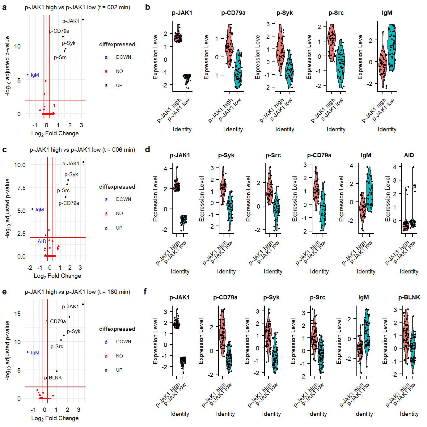
Suppl pJak1 High vs low
proteindata_counts <- as.data.frame(t(seu_combined_selectsamples@assays$PROT@scale.data)) %>%
  mutate(sample = rownames(t(seu_combined_selectsamples@assays$PROT@scale.data)))


metadata.all <- as.data.frame(seu_combined_selectsamples@meta.data) %>%
  mutate(sample = rownames((seu_combined_selectsamples@meta.data)))

proteindata_counts <- left_join(proteindata_counts, metadata.all)


toppJAK1 <- proteindata_counts %>%
  group_by(time) %>%
  top_frac(wt = `p-JAK1`, n = 0.05)

bottompJAK1 <- proteindata_counts %>%
  group_by(time) %>%
  top_frac(wt = `p-JAK1`, n = -0.05)

proteindata_counts <- proteindata_counts %>%
  mutate(highlowpJAK1 = ifelse(sample %in% toppJAK1$sample, "p-JAK1 high", ifelse(sample %in% bottompJAK1$sample, "p-JAK1 low","middle")))

addmeta <- proteindata_counts[,c("highlowpJAK1", "sample")]
rownames(addmeta) <- proteindata_counts$sample

seu_combined_selectsamples <- AddMetaData(seu_combined_selectsamples, addmeta)

seu.JAK1.180 <- subset(seu_combined_selectsamples, condition == "180.aIg.contr" & highlowpJAK1 != "middle")

seu.JAK1.180 <- SetIdent(seu.JAK1.180, value = "highlowpJAK1")
# Find differentially expressed features between CD14+ and FCGR3A+ Monocytes
markers.180 <- FindMarkers(seu.JAK1.180,ident.1 = "p-JAK1 high", ident.2 = "p-JAK1 low", assay = "PROT", slot = "scale.data", logfc.threshold = 0, return.thresh = 1, only.pos = F)
# view results
#markers.180 <- filter(markers.180, cluster == "p-JAK1 high")
#markers.180
# Find differentially expressed features between CD14+ and FCGR3A+ Monocytes
markers.180.RNA <- FindAllMarkers(seu.JAK1.180,assay = "RNA", slot = "data", logfc.threshold = 0.3, return.thresh = 0.01, only.pos = T,min.pct = 0.1)
markers.180.RNA <- FindMarkers(seu.JAK1.180,ident.1 = "p-JAK1 high", ident.2 = "p-JAK1 low", assay = "SCT.RNA", slot = "scale.data", logfc.threshold = 0, return.thresh = 1, only.pos = F)
# view results
#markers.180.RNA
markers.180$protein <-rownames(markers.180)
# add a column of NAs
markers.180$diffexpressed <- "NO"
# if log2Foldchange > 0.6 and pvalue < 0.05, set as "UP"
markers.180$diffexpressed[markers.180$avg_diff > 0.25 & markers.180$p_val_adj < 0.01] <- "UP"
# if log2Foldchange < -0.6 and pvalue < 0.05, set as "DOWN"
markers.180$diffexpressed[markers.180$avg_diff < -0.25 & markers.180$p_val_adj < 0.01] <- "DOWN"
mycolors <- c("blue", "red", "black")
names(mycolors) <- c("DOWN", "UP", "NO")
markers.180$delabel <- NA
markers.180$delabel[markers.180$diffexpressed != "NO"] <- markers.180$protein[markers.180$diffexpressed != "NO"]
# Finally, we can organize the labels nicely using the "ggrepel" package and the geom_text_repel() function
# load library
# plot adding up all layers we have seen so far
plot.vulcano.180min <- ggplot(data=markers.180, aes(x=avg_diff , y=-log10(p_val_adj), col=diffexpressed, label=delabel)) +
geom_point(size=0.5) +
theme_minimal() +
geom_text_repel(size=2.2) +
scale_color_manual(values=c("blue", "red", "black")) +
geom_vline(xintercept=c(-0.25, 0.25), col="red") +
geom_hline(yintercept=-log10(0.01), col="red") +
labs(x = expression("Log"[2]*" Fold Change"), y = expression("-log"[10]*" adjusted p-value"), title = "p-JAK1 high vs p-JAK1 low (t = 180 min)") &
add.textsize
sign.markers180 <- markers.180$protein[markers.180$avg_diff > 0.25 & markers.180$p_val_adj < 0.01 | markers.180$avg_diff < -0.25 & markers.180$p_val_adj < 0.01]
plot.vln.180min <- VlnPlot(seu.JAK1.180,assay = "PROT",slot = "scale.data", features = sign.markers180, group.by = "highlowpJAK1",ncol = 6, pt.size = 0.5) &
add.textsize
## RNA
markers.180.RNA$protein <-rownames(markers.180.RNA)
# add a column of NAs
markers.180.RNA$diffexpressed <- "NO"
# if log2Foldchange > 0.6 and pvalue < 0.05, set as "UP"
markers.180.RNA$diffexpressed[markers.180.RNA$avg_diff > 0.25 & markers.180.RNA$p_val < 0.05] <- "UP"
# if log2Foldchange < -0.6 and pvalue < 0.05, set as "DOWN"
markers.180.RNA$diffexpressed[markers.180.RNA$avg_diff < -0.25 & markers.180.RNA$p_val < 0.05] <- "DOWN"
mycolors <- c("blue", "red", "black")
names(mycolors) <- c("DOWN", "UP", "NO")
markers.180.RNA$delabel <- NA
markers.180.RNA$delabel[markers.180.RNA$diffexpressed != "NO"] <- markers.180.RNA$protein[markers.180.RNA$diffexpressed != "NO"]
# plot adding up all layers we have seen so far
plot.vulcano.180min.RNA <- ggplot(data=markers.180.RNA, aes(x=avg_diff, y=-log10(p_val), col=diffexpressed, label=delabel)) +
geom_point() +
theme_minimal() +
geom_text_repel(size=2.2) +
scale_color_manual(values=c("blue", "red", "black")) +
geom_vline(xintercept=c(-0.25, 0.25), col="red") +
geom_hline(yintercept=-log10(0.05), col="red") +
labs(x = expression("Log"[2]*" Fold Change"), y = expression("-log"[10]*" p-value"), title = "p-JAK1 high vs p-JAK1 low (t = 180 min)") &
add.textsize
sign.markers180.RNA <- markers.180.RNA$protein[markers.180.RNA$avg_diff > 0.25 & markers.180.RNA$p_val < 0.05]
plot.vln.180min.RNA <- VlnPlot(seu.JAK1.180,assay = "RNA", features = sign.markers180.RNA[1:20], group.by = "highlowpJAK1",ncol = 10) &
add.textsize
plot_180min <- plot_grid(plot.vulcano.180min, plot.vln.180min, labels = panellabels[c(5,6)], label_size = 10, ncol = 2, rel_widths = c(1,2))
## 6 minutes
seu.JAK1.006 <- subset(seu_combined_selectsamples, condition == "006.aIg.contr" & highlowpJAK1 != "middle")
seu.JAK1.006 <- SetIdent(seu.JAK1.006, value = "highlowpJAK1")
# Find differentially expressed features between CD14+ and FCGR3A+ Monocytes
markers.006 <- FindMarkers(seu.JAK1.006,ident.1 = "p-JAK1 high", ident.2 = "p-JAK1 low", assay = "PROT", slot = "scale.data", logfc.threshold = 0, return.thresh = 1, only.pos = F)
# view results
#markers.006 <- filter(markers.006, cluster == "p-JAK1 high")
#markers.006
# Find differentially expressed features between CD14+ and FCGR3A+ Monocytes
markers.006.RNA <- FindAllMarkers(seu.JAK1.006,assay = "RNA", slot = "data", logfc.threshold = 0.3, return.thresh = 0.01, only.pos = T,min.pct = 0.1)
markers.006.RNA <- FindMarkers(seu.JAK1.006,ident.1 = "p-JAK1 high", ident.2 = "p-JAK1 low", assay = "SCT.RNA", slot = "scale.data", logfc.threshold = 0, return.thresh = 1, only.pos = F)
# view results
#markers.006.RNA
markers.006$protein <-rownames(markers.006)
# add a column of NAs
markers.006$diffexpressed <- "NO"
# if log2Foldchange > 0.6 and pvalue < 0.05, set as "UP"
markers.006$diffexpressed[markers.006$avg_diff > 0.25 & markers.006$p_val_adj < 0.01] <- "UP"
# if log2Foldchange < -0.6 and pvalue < 0.05, set as "DOWN"
markers.006$diffexpressed[markers.006$avg_diff < -0.25 & markers.006$p_val_adj < 0.01] <- "DOWN"
mycolors <- c("blue", "red", "black")
names(mycolors) <- c("DOWN", "UP", "NO")
markers.006$delabel <- NA
markers.006$delabel[markers.006$diffexpressed != "NO"] <- markers.006$protein[markers.006$diffexpressed != "NO"]
# Finally, we can organize the labels nicely using the "ggrepel" package and the geom_text_repel() function
# load library
# plot adding up all layers we have seen so far
plot.vulcano.006min <- ggplot(data=markers.006, aes(x=avg_diff , y=-log10(p_val_adj), col=diffexpressed, label=delabel)) +
geom_point(size=0.5) +
theme_minimal() +
geom_text_repel(size=2.2) +
scale_color_manual(values=c("blue", "red", "black")) +
geom_vline(xintercept=c(-0.25, 0.25), col="red") +
geom_hline(yintercept=-log10(0.01), col="red") +
labs(x = expression("Log"[2]*" Fold Change"), y = expression("-log"[10]*" adjusted p-value"), title = "p-JAK1 high vs p-JAK1 low (t = 006 min)") &
add.textsize
sign.markers006 <- markers.006$protein[markers.006$avg_diff > 0.25 & markers.006$p_val_adj < 0.01 | markers.006$avg_diff < -0.25 & markers.006$p_val_adj < 0.01]
plot.vln.006min <- VlnPlot(seu.JAK1.006,assay = "PROT",slot = "scale.data", features = sign.markers006, group.by = "highlowpJAK1",ncol = 6, pt.size = 0.5) &
add.textsize
markers.006.RNA$protein <-rownames(markers.006.RNA)
# add a column of NAs
markers.006.RNA$diffexpressed <- "NO"
# if log2Foldchange > 0.6 and pvalue < 0.05, set as "UP"
markers.006.RNA$diffexpressed[markers.006.RNA$avg_diff > 0.25 & markers.006.RNA$p_val < 0.05] <- "UP"
# if log2Foldchange < -0.6 and pvalue < 0.05, set as "DOWN"
markers.006.RNA$diffexpressed[markers.006.RNA$avg_diff < -0.25 & markers.006.RNA$p_val < 0.05] <- "DOWN"
mycolors <- c("blue", "red", "black")
names(mycolors) <- c("DOWN", "UP", "NO")
markers.006.RNA$delabel <- NA
markers.006.RNA$delabel[markers.006.RNA$diffexpressed != "NO"] <- markers.006.RNA$protein[markers.006.RNA$diffexpressed != "NO"]
# Finally, we can organize the labels nicely using the "ggrepel" package and the geom_text_repel() function
# load library
# plot adding up all layers we have seen so far
plot.vulcano.006min.RNA <- ggplot(data=markers.006.RNA, aes(x=avg_diff, y=-log10(p_val), col=diffexpressed, label=delabel)) +
geom_point() +
theme_minimal() +
geom_text_repel(size=2.2) +
scale_color_manual(values=c("blue", "red", "black")) +
geom_vline(xintercept=c(-0.25, 0.25), col="red") +
geom_hline(yintercept=-log10(0.05), col="red") +
labs(x = expression("Log"[2]*" Fold Change"), y = expression("-log"[10]*" p-value"), title = "p-JAK1 high vs p-JAK1 low (t = 006 min)") &
add.textsize
sign.markers006.RNA <- markers.006.RNA$protein[markers.006.RNA$avg_diff > 0.25 & markers.006.RNA$p_val < 0.05]
plot.vln.006min.RNA <- VlnPlot(seu.JAK1.006,assay = "RNA", features = sign.markers006.RNA[1:20], group.by = "highlowpJAK1",ncol = 10) &
add.textsize
plot_006min <- plot_grid(plot.vulcano.006min, plot.vln.006min, labels = panellabels[c(3,4)], label_size = 10, ncol = 2, rel_widths = c(1,2))
## 2 minutes
seu.JAK1.002 <- subset(seu_combined_selectsamples, condition == "002.aIg.contr" & highlowpJAK1 != "middle")
seu.JAK1.002 <- SetIdent(seu.JAK1.002, value = "highlowpJAK1")
# Find differentially expressed features between CD14+ and FCGR3A+ Monocytes
markers.002 <- FindMarkers(seu.JAK1.002,ident.1 = "p-JAK1 high", ident.2 = "p-JAK1 low", assay = "PROT", slot = "scale.data", logfc.threshold = 0, return.thresh = 1, only.pos = F)
# view results
#markers.002 <- filter(markers.002, cluster == "p-JAK1 high")
#markers.002
# Find differentially expressed features between CD14+ and FCGR3A+ Monocytes
markers.002.RNA <- FindAllMarkers(seu.JAK1.002,assay = "RNA", slot = "data", logfc.threshold = 0.3, return.thresh = 0.01, only.pos = T,min.pct = 0.1)
markers.002.RNA <- FindMarkers(seu.JAK1.002,ident.1 = "p-JAK1 high", ident.2 = "p-JAK1 low", assay = "SCT.RNA", slot = "scale.data", logfc.threshold = 0, return.thresh = 1, only.pos = F)
# view results
#markers.002.RNA
markers.002$protein <-rownames(markers.002)
# add a column of NAs
markers.002$diffexpressed <- "NO"
# if log2Foldchange > 0.6 and pvalue < 0.05, set as "UP"
markers.002$diffexpressed[markers.002$avg_diff > 0.25 & markers.002$p_val_adj < 0.01] <- "UP"
# if log2Foldchange < -0.6 and pvalue < 0.05, set as "DOWN"
markers.002$diffexpressed[markers.002$avg_diff < -0.25 & markers.002$p_val_adj < 0.01] <- "DOWN"
mycolors <- c("blue", "red", "black")
names(mycolors) <- c("DOWN", "UP", "NO")
markers.002$delabel <- NA
markers.002$delabel[markers.002$diffexpressed != "NO"] <- markers.002$protein[markers.002$diffexpressed != "NO"]
plot.vulcano.002min <- ggplot(data=markers.002, aes(x=avg_diff , y=-log10(p_val_adj), col=diffexpressed, label=delabel)) +
geom_point(size=0.5) +
theme_minimal() +
geom_text_repel(size=2.2) +
scale_color_manual(values=c("blue", "red", "black")) +
geom_vline(xintercept=c(-0.25, 0.25), col="red") +
geom_hline(yintercept=-log10(0.01), col="red") +
labs(x = expression("Log"[2]*" Fold Change"), y = expression("-log"[10]*" adjusted p-value"), title = "p-JAK1 high vs p-JAK1 low (t = 002 min)") &
add.textsize
sign.markers002 <- markers.002$protein[markers.002$avg_diff > 0.25 & markers.002$p_val_adj < 0.01 | markers.002$avg_diff < -0.25 & markers.002$p_val_adj < 0.01]
plot.vln.002min <- VlnPlot(seu.JAK1.002,assay = "PROT",slot = "scale.data", features = sign.markers002, group.by = "highlowpJAK1",ncol = 6, pt.size = 0.5) &
add.textsize
markers.002.RNA$protein <-rownames(markers.002.RNA)
# add a column of NAs
markers.002.RNA$diffexpressed <- "NO"
# if log2Foldchange > 0.6 and pvalue < 0.05, set as "UP"
markers.002.RNA$diffexpressed[markers.002.RNA$avg_diff > 0.25 & markers.002.RNA$p_val < 0.05] <- "UP"
# if log2Foldchange < -0.6 and pvalue < 0.05, set as "DOWN"
markers.002.RNA$diffexpressed[markers.002.RNA$avg_diff < -0.25 & markers.002.RNA$p_val < 0.05] <- "DOWN"
mycolors <- c("blue", "red", "black")
names(mycolors) <- c("DOWN", "UP", "NO")
markers.002.RNA$delabel <- NA
markers.002.RNA$delabel[markers.002.RNA$diffexpressed != "NO"] <- markers.002.RNA$protein[markers.002.RNA$diffexpressed != "NO"]
plot.vulcano.002min.RNA <- ggplot(data=markers.002.RNA, aes(x=avg_diff, y=-log10(p_val), col=diffexpressed, label=delabel)) +
geom_point() +
theme_minimal() +
geom_text_repel(size=2.2) +
scale_color_manual(values=c("blue", "red", "black")) +
geom_vline(xintercept=c(-0.25, 0.25), col="red") +
geom_hline(yintercept=-log10(0.05), col="red") +
labs(x = expression("Log"[2]*" Fold Change"), y = expression("-log"[10]*" p-value"), title = "p-JAK1 high vs p-JAK1 low (t = 002 min)") &
add.textsize
sign.markers002.RNA <- markers.002.RNA$protein[markers.002.RNA$avg_diff > 0.25 & markers.002.RNA$p_val < 0.05]
plot.vln.002min.RNA <- VlnPlot(seu.JAK1.002,assay = "RNA", features = sign.markers002.RNA[1:20], group.by = "highlowpJAK1",ncol = 10) &
add.textsize
plot_002min <- plot_grid(plot.vulcano.002min, plot.vln.002min, labels = panellabels[c(1,2)], label_size = 10, ncol = 2, rel_widths = c(1,2))plot_all <- plot_grid(plot_002min,plot_006min,plot_180min , labels =c("", "", ""), ncol = 1, rel_heights = c(1,1,1))
ggsave(plot_all, filename = "output/paper_figures/Suppl_pJAK1_highlow.pdf", width = 183, height = 140, units = "mm", dpi = 300, useDingbats = FALSE)
ggsave(plot_all, filename = "output/paper_figures/Suppl_pJAK1_highlow.png", width = 183, height = 140, units = "mm", dpi = 300)
plot_all
sessionInfo()R version 4.0.3 (2020-10-10)
Platform: x86_64-w64-mingw32/x64 (64-bit)
Running under: Windows 10 x64 (build 19042)
Matrix products: default
locale:
[1] LC_COLLATE=English_Netherlands.1252 LC_CTYPE=English_Netherlands.1252
[3] LC_MONETARY=English_Netherlands.1252 LC_NUMERIC=C
[5] LC_TIME=English_Netherlands.1252
attached base packages:
[1] parallel stats4 grid stats graphics grDevices utils
[8] datasets methods base
other attached packages:
[1] png_0.1-7 forcats_0.5.1
[3] clusterProfiler_3.18.1 clusterProfiler.dplyr_0.0.2
[5] enrichplot_1.10.2 org.Hs.eg.db_3.12.0
[7] AnnotationDbi_1.52.0 IRanges_2.24.1
[9] S4Vectors_0.28.1 Biobase_2.50.0
[11] BiocGenerics_0.36.0 ggridges_0.5.3
[13] cowplot_1.1.1 ggtext_0.1.1
[15] ggplotify_0.0.5 ggcorrplot_0.1.3
[17] ggrepel_0.9.1 ggpubr_0.4.0
[19] scico_1.2.0 MOFA2_1.1.17
[21] extrafont_0.17 patchwork_1.1.1
[23] RColorBrewer_1.1-2 viridis_0.5.1
[25] viridisLite_0.3.0 ggsci_2.9
[27] sctransform_0.3.2 ggthemes_4.2.4
[29] matrixStats_0.57.0 kableExtra_1.3.1
[31] gridExtra_2.3 SeuratObject_4.0.0
[33] Seurat_4.0.0 ggplot2_3.3.3
[35] scales_1.1.1 tidyr_1.1.2
[37] dplyr_1.0.3 stringr_1.4.0
[39] workflowr_1.6.2
loaded via a namespace (and not attached):
[1] rappdirs_0.3.2 scattermore_0.7 bit64_4.0.5
[4] knitr_1.31 irlba_2.3.3 DelayedArray_0.16.1
[7] data.table_1.13.6 rpart_4.1-15 generics_0.1.0
[10] RSQLite_2.2.3 shadowtext_0.0.7 RANN_2.6.1
[13] future_1.21.0 bit_4.0.4 spatstat.data_2.1-0
[16] webshot_0.5.2 xml2_1.3.2 httpuv_1.5.5
[19] assertthat_0.2.1 xfun_0.23 hms_1.0.0
[22] evaluate_0.14 promises_1.1.1 readxl_1.3.1
[25] tmvnsim_1.0-2 igraph_1.2.6 DBI_1.1.1
[28] htmlwidgets_1.5.3 purrr_0.3.4 ellipsis_0.3.1
[31] RSpectra_0.16-0 corrplot_0.84 backports_1.2.1
[34] markdown_1.1 deldir_0.2-10 MatrixGenerics_1.2.0
[37] vctrs_0.3.6 ROCR_1.0-11 abind_1.4-5
[40] cachem_1.0.1 withr_2.4.1 ggforce_0.3.2
[43] mnormt_2.0.2 goftest_1.2-2 cluster_2.1.0
[46] DOSE_3.16.0 lazyeval_0.2.2 crayon_1.3.4
[49] basilisk.utils_1.2.1 pkgconfig_2.0.3 labeling_0.4.2
[52] tweenr_1.0.1 nlme_3.1-149 rlang_0.4.10
[55] globals_0.14.0 lifecycle_0.2.0 miniUI_0.1.1.1
[58] downloader_0.4 filelock_1.0.2 extrafontdb_1.0
[61] cellranger_1.1.0 rprojroot_2.0.2 polyclip_1.10-0
[64] lmtest_0.9-38 Matrix_1.2-18 carData_3.0-4
[67] Rhdf5lib_1.12.1 zoo_1.8-8 whisker_0.4
[70] pheatmap_1.0.12 KernSmooth_2.23-17 rhdf5filters_1.2.0
[73] blob_1.2.1 qvalue_2.22.0 parallelly_1.23.0
[76] rstatix_0.6.0 gridGraphics_0.5-1 ggsignif_0.6.0
[79] memoise_2.0.0 magrittr_2.0.1 plyr_1.8.6
[82] ica_1.0-2 compiler_4.0.3 scatterpie_0.1.5
[85] fitdistrplus_1.1-3 listenv_0.8.0 pbapply_1.4-3
[88] MASS_7.3-53 mgcv_1.8-33 tidyselect_1.1.0
[91] stringi_1.5.3 highr_0.8 yaml_2.2.1
[94] GOSemSim_2.16.1 fastmatch_1.1-0 tools_4.0.3
[97] future.apply_1.7.0 rio_0.5.16 rstudioapi_0.13
[100] foreign_0.8-80 git2r_0.28.0 farver_2.0.3
[103] Rtsne_0.15 ggraph_2.0.5 digest_0.6.27
[106] rvcheck_0.1.8 BiocManager_1.30.10 shiny_1.6.0
[109] Rcpp_1.0.6 gridtext_0.1.4 car_3.0-10
[112] broom_0.7.3 later_1.1.0.1 RcppAnnoy_0.0.18
[115] httr_1.4.2 psych_2.0.12 colorspace_2.0-0
[118] rvest_0.3.6 fs_1.5.0 tensor_1.5
[121] reticulate_1.18 splines_4.0.3 uwot_0.1.10
[124] spatstat.utils_2.1-0 graphlayouts_0.7.1 basilisk_1.2.1
[127] plotly_4.9.3 xtable_1.8-4 jsonlite_1.7.2
[130] spatstat_1.64-1 tidygraph_1.2.0 R6_2.5.0
[133] pillar_1.4.7 htmltools_0.5.1.1 mime_0.9
[136] glue_1.4.2 fastmap_1.1.0 BiocParallel_1.24.1
[139] codetools_0.2-16 fgsea_1.16.0 lattice_0.20-41
[142] tibble_3.0.5 curl_4.3 leiden_0.3.7
[145] zip_2.1.1 GO.db_3.12.1 openxlsx_4.2.3
[148] Rttf2pt1_1.3.8 limma_3.46.0 survival_3.2-7
[151] rmarkdown_2.6 munsell_0.5.0 DO.db_2.9
[154] rhdf5_2.34.0 HDF5Array_1.18.0 haven_2.3.1
[157] reshape2_1.4.4 gtable_0.3.0
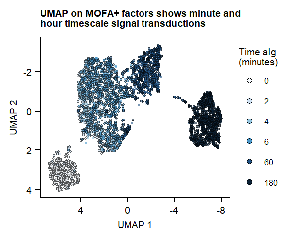 Figure 1. UMAP of 7 MOFA factors, integrating phospho-protein and RNA measurements
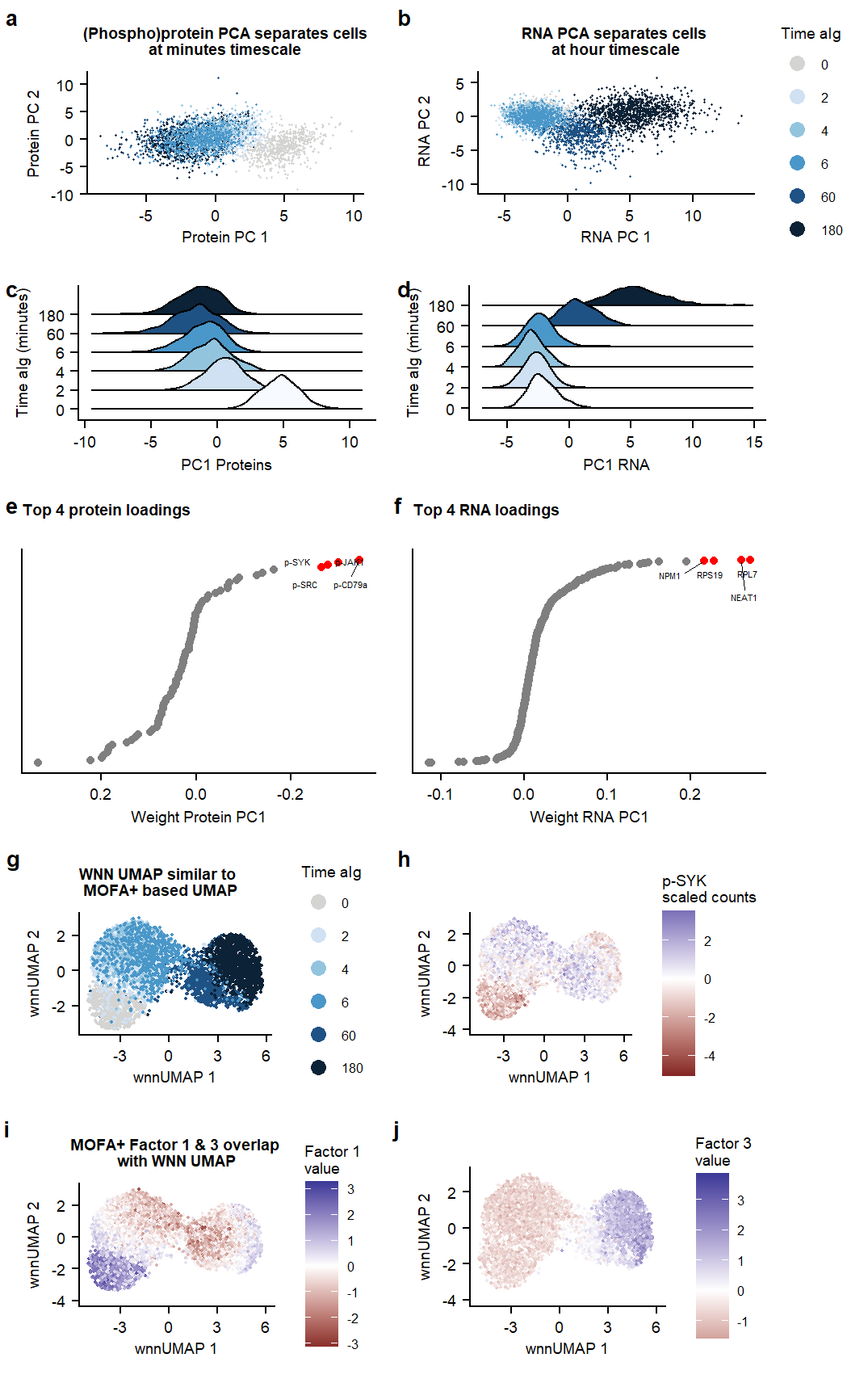 Supplementary Figure. PCA analysis on RNA and Protein datasets separately.
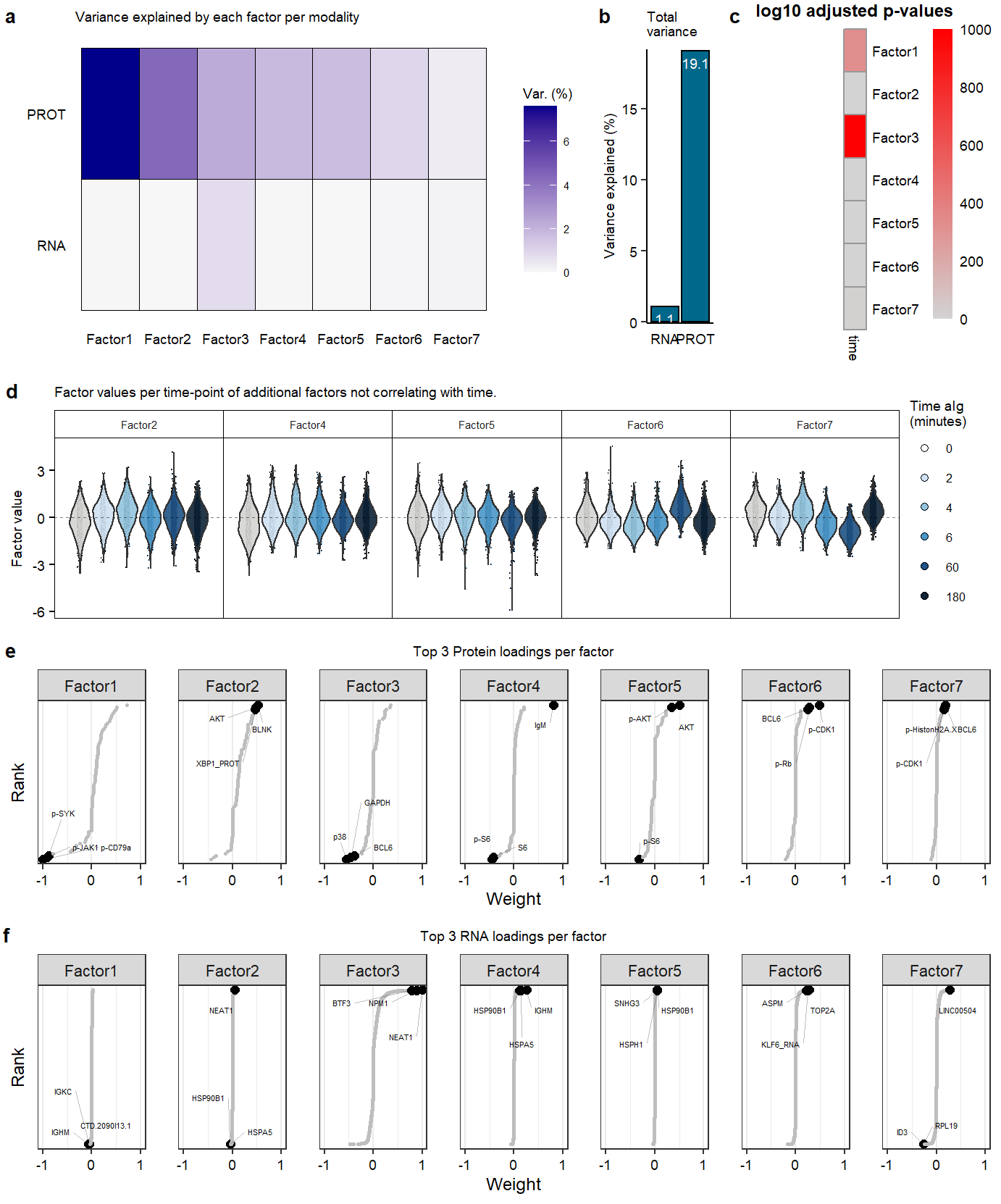 Supplementary Figure. MOFA model additional information
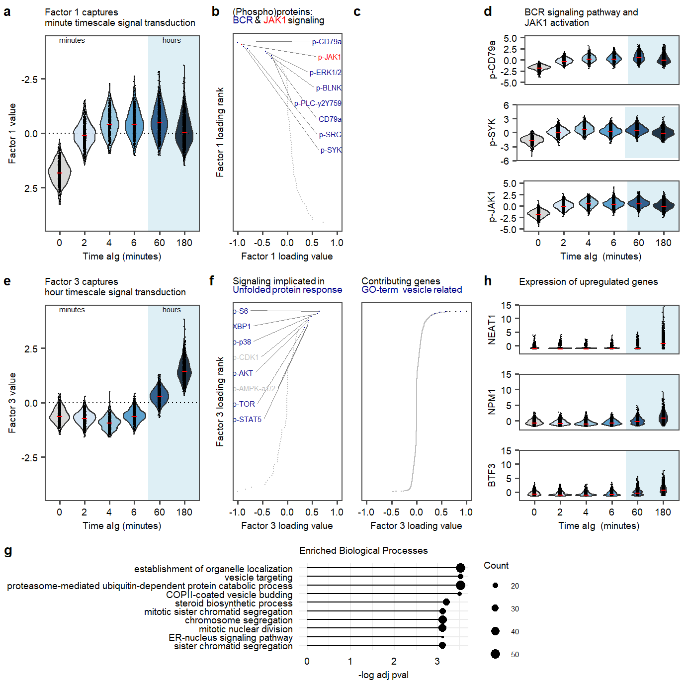 Figure 2. Factor 1 and 3 exploration.
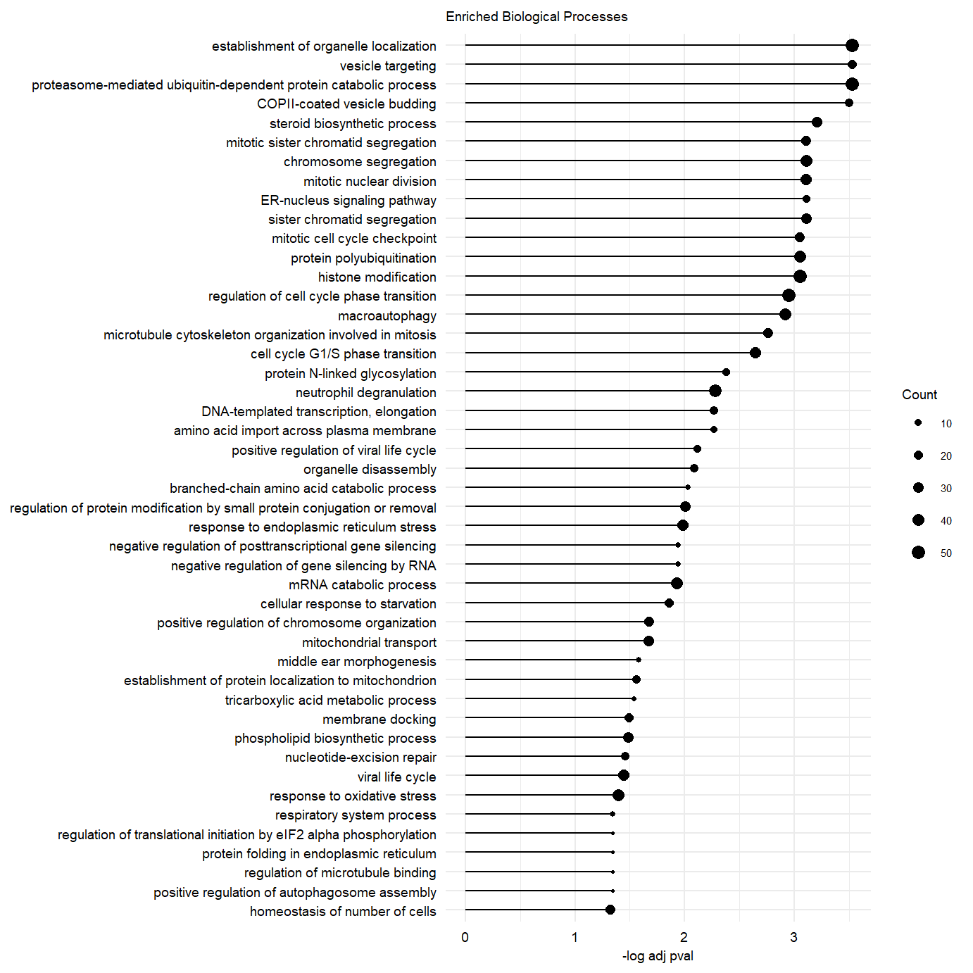 Supplementary Figure. Top 50 enriched gene-sets in postive loadings factor 3.