Hallmark Ig-classes

workflowr

• Summary
• Checks
• Past versions

Last updated: 2023-01-17

Checks: 7 0

Knit directory: Multimodal-Plasmacell_manuscript/

This reproducible R Markdown analysis was created with workflowr (version 1.6.2). The Checks tab describes the reproducibility checks that were applied when the results were created. The Past versions tab lists the development history.

---

R Markdown file: up-to-date

Great! Since the R Markdown file has been committed to the Git repository, you know the exact version of the code that produced these results.

Environment: empty

Great job! The global environment was empty. Objects defined in the global environment can affect the analysis in your R Markdown file in unknown ways. For reproduciblity it’s best to always run the code in an empty environment.

Seed: set.seed(20211005)

The command set.seed(20211005) was run prior to running the code in the R Markdown file. Setting a seed ensures that any results that rely on randomness, e.g. subsampling or permutations, are reproducible.

Session information: recorded

Great job! Recording the operating system, R version, and package versions is critical for reproducibility.

Cache: none

Nice! There were no cached chunks for this analysis, so you can be confident that you successfully produced the results during this run.

File paths: relative

Great job! Using relative paths to the files within your workflowr project makes it easier to run your code on other machines.

Repository version: 95e922e

Great! You are using Git for version control. Tracking code development and connecting the code version to the results is critical for reproducibility.

The results in this page were generated with repository version 95e922e. See the Past versions tab to see a history of the changes made to the R Markdown and HTML files.

Note that you need to be careful to ensure that all relevant files for the analysis have been committed to Git prior to generating the results (you can use wflow_publish or wflow_git_commit). workflowr only checks the R Markdown file, but you know if there are other scripts or data files that it depends on. Below is the status of the Git repository when the results were generated:

Ignored files:
    Ignored:    .Rhistory
    Ignored:    .Rproj.user/
    Ignored:    analysis/cellstate_sidetest.Rmd
    Ignored:    analysis/hallmarks2.Rmd
    Ignored:    analysis/supplements.Rmd
    Ignored:    data/Seq2Science/
    Ignored:    data/azimuth_PBMCs/
    Ignored:    data/azimuth_bonemarrow/
    Ignored:    data/citeseqcount_htseqcount.zip
    Ignored:    data/genelist.plots.diffmarkers.txt
    Ignored:    data/genelist.plots.diffmarkers2.txt
    Ignored:    data/raw/
    Ignored:    data/supplementary/
    Ignored:    output/MOFA_analysis_Donorgroup.hdf5
    Ignored:    output/MOFA_analysis_Donorgroup.rds
    Ignored:    output/MOFA_analysis_Donorgroup_clustered.rds
    Ignored:    output/MOFA_analysis_Donorgroup_noIg.hdf5
    Ignored:    output/MOFA_analysis_Donorgroup_noIg2.hdf5
    Ignored:    output/extra plots.docx
    Ignored:    output/paper_figures/
    Ignored:    output/seu.fix_norm.rds
    Ignored:    output/seu.fix_norm_cellstate.rds
    Ignored:    output/seu.fix_norm_plasmacells.rds
    Ignored:    output/seu.live_norm.rds
    Ignored:    output/seu.live_norm_cellstate.rds
    Ignored:    output/seu.live_norm_plasmacells.rds
    Ignored:    output/seu.live_norm_plasmacells_RNA.rds
    Ignored:    output/top-PROT-loadings_IgA.tsv
    Ignored:    output/top-PROT-loadings_IgG.tsv
    Ignored:    output/top-PROT-loadings_IgM.tsv
    Ignored:    output/top-gene-loadings_IgA.tsv
    Ignored:    output/top-gene-loadings_IgG.tsv
    Ignored:    output/top-gene-loadings_IgM.csv
    Ignored:    output/top-gene-loadings_IgM.tsv

Unstaged changes:
    Modified:   .gitignore
    Modified:   CITATION.bib

Note that any generated files, e.g. HTML, png, CSS, etc., are not included in this status report because it is ok for generated content to have uncommitted changes.

---

These are the previous versions of the repository in which changes were made to the R Markdown (analysis/hallmarks.Rmd) and HTML (docs/hallmarks.html) files. If you’ve configured a remote Git repository (see ?wflow_git_remote), click on the hyperlinks in the table below to view the files as they were in that past version.

File	Version	Author	Date	Message
Rmd	95e922e	Jessie van Buggenum	2023-01-17	final docs

---

seu.fix <- readRDS( file = "output/seu.fix_norm_plasmacells.rds")
seu.fix <- SetIdent(seu.fix,value = "IgClass")
Idents(seu.fix) <- factor(x = Idents(seu.fix), levels = c("IgM", "IgG", "IgA"))

seu.live <- readRDS(file = "output/seu.live_norm_plasmacells.rds")
seu.live <-SetIdent(seu.live,value = "IgClass")
Idents(seu.live) <- factor(x = Idents(seu.live), levels = c("IgM", "IgG", "IgA"))

To explore differences between three Ig-classes, we analyse protein and gene weights from the MOFA model and determine differential expressed genes or proteins.

# Read in the MOFA analysis file
mofa <- readRDS(file= "output/MOFA_analysis_Donorgroup_clustered.rds")

### Get all weights 
weights.RNA <- get_weights(mofa, views = "RNA",as.data.frame = TRUE)

weights.PROT.fix <- get_weights(mofa, views = "PROT.fix",as.data.frame = TRUE) %>%
  mutate(feature = gsub('.{2}$',x =  feature, replacement = '') )
weights.PROT.live <- get_weights(mofa, views = "PROT.live",as.data.frame = TRUE) %>%
  mutate(feature = gsub('.{2}$',x =  feature, replacement = '') )
weights.PROT.common <- get_weights(mofa, views = "PROT.common",as.data.frame = TRUE)

weights.protein <- rbind(weights.PROT.common,weights.PROT.live,weights.PROT.fix) %>%
  filter(factor == "Factor1" | factor == "Factor2") %>%
  spread(factor,value)

# Define lists of B cell selection, homing selection and diffgenes and diffprots
list.Bcell.selection <- c("CD25", "CD32", "CD20","CD19", "CD22", "CD40", "CD86") 
list.Bcell.selection.f <- c( "IgD", "CD23", "CD5", "CD70")
list.homing.selection.f <- c("CXCR4", "CXCR5","IntegrinA4")
list.homing.selection <- c("IntegrinB7", "IntegrinB1","CD49d", "CCR9", "CD31", "CD44","CXCR3")
list.Bcell.selection.new <- c( "CD138", "CD38", "CD27", "CD20","CD19")

# Read in the genelist for plots
genelist_plots_diffmarkers <- read_delim("data/genelist.plots.diffmarkers2.txt", 
    "\t", escape_double = FALSE, trim_ws = TRUE)

# Extract diffgenes and diffprots
list.genes.select.diffgenes <- c(unique(subset(genelist_plots_diffmarkers, modality == "RNA")$gene))
list.prot.select.diffprots <- c(unique(subset(genelist_plots_diffmarkers,  modality == "PROT")$gene))

# Concatenate the lists
list.dotplot.prots <- c(list.prot.select.diffprots,list.homing.selection,list.homing.selection.f,list.Bcell.selection.f,list.Bcell.selection)

# Add a new column with feature to plot
weights.protein <- weights.protein %>%
  mutate(features.toplot = ifelse(feature %in% c(list.dotplot.prots, "IgM", "IgA", "IgG"),as.character(feature),""))

Fig.3

view.labs <- c("Common proteins", "Live-cell proteins", "Fixed-cell proteins")
names(view.labs) <- c("PROT.common", "PROT.live", "PROT.fix")

p.loadings.scatter.prot <- 
ggplot(weights.protein, aes(Factor1, Factor2)) +
    geom_hline(yintercept = 0, color = "grey", alpha = 0.8)+
      geom_vline(xintercept = 0, color = "grey", alpha = 0.8)+
  geom_point(size = 0.5) +
  facet_wrap(~view,
              labeller = labeller(view = view.labs),
             scales = "free") +
  theme_few()+
  ggrepel::geom_text_repel( data          = subset(weights.protein, Factor1 > 10^-2 ),
                            aes(x=Factor1, y=Factor2, label=feature), size=1.8, max.overlaps = Inf,
     segment.size  = 0.15,
    segment.color = "grey50",
    direction     = "y",
    hjust         = 0)+
  
      ggrepel::geom_text_repel(
    data          = subset(weights.protein, Factor1 < -10^-2& Factor2 >10^-2 ),
    aes(x=Factor1, y=Factor2, label=feature), size=1.8, max.overlaps = Inf,
      segment.size  = 0.15,
    segment.color = "grey50",
    direction     = "y",
    hjust         = 1
  ) +
      ggrepel::geom_text_repel(
    data          = subset(weights.protein, Factor1 < -10^-2 & Factor2 <10^-2),
    aes(x=Factor1, y=Factor2, label=feature), size=1.8, max.overlaps = Inf,
     segment.size  = 0.15,
    segment.color = "grey50",
    direction     = "y",
    hjust         = 1
  )+
     add.textsize   +
    labs(title = "Protein loading values contributing to Factor 1 and 2\nrepresent IgM, IgG or IgA associated (phospho-)proteins ") +
  theme(
        panel.grid.major = element_blank(),
    panel.grid.minor = element_blank())

# p.loadings.scatter.prot

topposrna.factor1.IgA <-  weights.RNA %>%
    spread(factor, value) %>%
  filter(Factor1 >= 10^-8) %>%
  select(c(feature, Factor1, Factor2)) %>%
  mutate(sortFactor1 = Factor1) %>%
  arrange(-sortFactor1)
  
rownames(topposrna.factor1.IgA) <- topposrna.factor1.IgA$feature

topposPROT.fix.factor1.IgA <- weights.PROT.fix %>%
    spread(factor, value) %>%
  filter(Factor1 >= 10^-8) %>%
  arrange(-Factor1)
rownames(topposPROT.fix.factor1.IgA) <- topposPROT.fix.factor1.IgA$feature

topposPROT.live.factor1.IgA <- weights.PROT.live %>%
    spread(factor, value) %>%
  filter(Factor1 >= 10^-8) %>%
  arrange(-Factor1)
rownames(topposPROT.live.factor1.IgA) <- topposPROT.live.factor1.IgA$feature

topposPROT.common.factor1.IgA <- weights.PROT.common %>%
    spread(factor, value) %>%
  filter(Factor1 >= 10^-8) %>%
  arrange(-Factor1)
rownames(topposPROT.common.factor1.IgA) <- topposPROT.common.factor1.IgA$feature


loadings.prot.IgA <- rbind(topposPROT.fix.factor1.IgA,topposPROT.live.factor1.IgA,topposPROT.common.factor1.IgA)
loadings.prot.IgA <- arrange(loadings.prot.IgA, -Factor1)

topnegrna.factor2.IgM <- weights.RNA %>%
    spread(factor, value) %>%
  filter(Factor1 <= -10^-8) %>%
  filter(Factor2 <= -10^-8) %>%
  select(c(feature, Factor1, Factor2)) %>%
  mutate(sortminusFactor1times2 = -(Factor2*Factor1)) %>%
  arrange(sortminusFactor1times2)

rownames(topnegrna.factor2.IgM) <- topnegrna.factor2.IgM$feature

##filter for not IgA
##filter for not IgA
#topnegrna.factor2.IgM <-topnegrna.factor2.IgM[topnegrna.factor2.IgM$feature %in% topnegrna.factor1.IgMIgG$feature,]

topnegPROT.fix.factor2.IgM <- weights.PROT.fix %>%
  spread(factor, value) %>%
  filter(Factor1 <= -10^-7) %>%
  filter(Factor2 <= -10^-7) %>%
   arrange(Factor2)
rownames(topnegPROT.fix.factor2.IgM) <- topnegPROT.fix.factor2.IgM$feature

topnegPROT.live.factor2.IgM <- weights.PROT.live %>%
  spread(factor, value) %>%
  filter(Factor1 <= -10^-7) %>%
  filter(Factor2 <= -10^-7) %>%
  arrange(Factor2) 

rownames(topnegPROT.live.factor2.IgM) <- topnegPROT.live.factor2.IgM$feature

topnegPROT.common.factor2.IgM <- weights.PROT.common %>%
  spread(factor, value) %>%
  filter(Factor1 <= -10^-7) %>%
  filter(Factor2 <= -10^-7) %>%
  arrange(Factor2)
rownames(topnegPROT.common.factor2.IgM) <- topnegPROT.common.factor2.IgM$feature

loadings.prot.IgM <- rbind(topnegPROT.fix.factor2.IgM,topnegPROT.live.factor2.IgM,topnegPROT.common.factor2.IgM)
loadings.prot.IgM <- arrange(loadings.prot.IgM, -(Factor2*Factor1) )

topposrna.factor2.IgG <-weights.RNA %>%
    spread(factor, value) %>%
  filter(Factor1 <= -10^-8) %>%
  filter(Factor2 >= 10^-8) %>%
  select(c(feature, Factor1, Factor2)) %>%
  mutate(sortFactor2timesminus1 =  -(Factor2*-Factor1)) %>%
  arrange(sortFactor2timesminus1)
rownames(topposrna.factor2.IgG) <- topposrna.factor2.IgG$feature
##filter for not IgA
#topposrna.factor2.IgG <-topposrna.factor2.IgG[topposrna.factor2.IgG$feature %in% topnegrna.factor1.IgMIgG$feature,]

topposPROT.fix.factor2.IgG <- weights.PROT.fix %>%
    spread(factor, value) %>%
  filter(Factor1 <= -10^-7) %>%
  filter(Factor2 >= 10^-7) %>%
  arrange(-Factor2) 

rownames(topposPROT.fix.factor2.IgG) <- topposPROT.fix.factor2.IgG$feature

topposPROT.live.factor2.IgG <- weights.PROT.live %>%
    spread(factor, value) %>%
  filter(Factor1 <= -10^-7) %>%
  filter(Factor2 >= 10^-7) %>%
  arrange(-Factor2) 

rownames(topposPROT.live.factor2.IgG) <- topposPROT.live.factor2.IgG$feature

topposPROT.common.factor2.IgG <- weights.PROT.common %>%
    spread(factor, value) %>%
  filter(Factor1 <= -10^-7) %>%
  filter(Factor2 >= 10^-7) %>%
  arrange(-Factor2)
rownames(topposPROT.common.factor2.IgG) <- topposPROT.common.factor2.IgG$feature

loadings.prot.IgG <- rbind(topposPROT.fix.factor2.IgG,topposPROT.live.factor2.IgG,topposPROT.common.factor2.IgG)
loadings.prot.IgG <- arrange(loadings.prot.IgG, -(Factor2*-Factor1))

loadings.prot.IgM <- select(loadings.prot.IgM, c(feature, view, Factor1, Factor2))
loadings.prot.IgG <- select(loadings.prot.IgG, c(feature, view, Factor1, Factor2))
loadings.prot.IgA <- select(loadings.prot.IgA, c(feature, view, Factor1, Factor2))

# write_tsv(loadings.prot.IgM, file = "output/top-PROT-loadings_IgM.tsv")
# write_tsv(loadings.prot.IgA, file = "output/top-PROT-loadings_IgA.tsv")
# write_tsv(loadings.prot.IgG, file = "output/top-PROT-loadings_IgG.tsv")

# write_tsv(topnegrna.factor2.IgM, file = "output/top-gene-loadings_IgM.tsv")
# write_tsv(topposrna.factor1.IgA, file = "output/top-gene-loadings_IgA.tsv")
# write_tsv(topposrna.factor2.IgG, file = "output/top-gene-loadings_IgG.tsv")

list.genes.loadings.top20 <- rev(c(as.character(topnegrna.factor2.IgM$feature[1:20]),as.character(topposrna.factor1.IgA$feature[1:20]),as.character(topposrna.factor2.IgG$feature[1:20])))

list.genes.loadings.top200 <- rev(c(as.character(topnegrna.factor2.IgM$feature[1:200]),as.character(topposrna.factor2.IgG$feature[1:200]), as.character(topposrna.factor1.IgA$feature[1:200])))

list.genes.loadings.top200 <- rev(c(as.character(topnegrna.factor2.IgM$feature[1:200]),as.character(topposrna.factor2.IgG$feature[1:200]), as.character(topposrna.factor1.IgA$feature[1:200])))

list.genes.loadings.all <- rev(c(as.character(topnegrna.factor2.IgM$feature),as.character(topposrna.factor2.IgG$feature), as.character(topposrna.factor1.IgA$feature)))

All.diff.PROT.live <- unique(c(as.character(loadings.prot.IgM$feature),as.character(loadings.prot.IgG$feature),as.character(loadings.prot.IgA$feature)))
All.diff.PROT.fix <- unique(c(as.character(loadings.prot.IgM$feature),as.character(loadings.prot.IgG$feature),as.character(loadings.prot.IgA$feature)))

p.dotplot.Bcell.markers.l <- DotPlot(seu.live,assay = "PROT",features = rev(sort((All.diff.PROT.live[All.diff.PROT.live %in%list.Bcell.selection.new] ))), cols = "RdBu",dot.scale = 3, scale.min = 0, scale = T, scale.by = "size", col.min = -0.5, col.max = 0.5)+coord_flip() +
  labs(x = "Proteins \n(live)", y = "", title = "B-cell markers expression \nsurface-proteins") +
  add.textsize +
  theme(legend.position = "none", 
        legend.key.size = unit(2, 'mm'),
        axis.ticks.x=element_blank(),
        axis.text.y = element_text(angle=0, hjust=1))

p.dotplot.Bcell.markers.f <- DotPlot(seu.fix,assay = "PROT",features = rev(c(All.diff.PROT.fix[All.diff.PROT.fix%in%list.Bcell.selection.f] )) , cols = "RdBu",dot.scale = 3, scale.min = 0, scale = T, scale.by = "size", col.min = -0.5, col.max = 0.5)+coord_flip() +
  labs(x = "Proteins (fixed)", y = "") +
  add.textsize +
  theme(legend.position = "none", 
        legend.key.size = unit(2, 'mm'),
        axis.text.y = element_text(angle=0, hjust=1))



p.dotplot.gene.diff.gene <- DotPlot(seu.live,assay = "SCT",features =sort(unique(list.genes.loadings.all[list.genes.loadings.all %in%list.genes.select.diffgenes])) , cols = "RdBu",dot.scale = 3, scale.min = 0, scale.max = 100, scale = T, scale.by = "size", col.min = -0.5, col.max = 0.5)+coord_flip() +
  labs(x = "Selected differentiation \ngenes", y = "", title = "PC differentiation markers \nand regulators")  +
  add.textsize +
  theme(legend.position = "none", 
        axis.text.y = element_text(angle=0, hjust=1,face = "italic"), 
        legend.key.size = unit(2, 'mm'),
        axis.text.x = element_text(angle=0, hjust=0.5),
        legend.box="vertical", legend.margin=margin())

p.dotplot.gene.diff.prot.f <- DotPlot(seu.fix,assay = "PROT",features = sort((All.diff.PROT.fix[All.diff.PROT.fix%in%list.prot.select.diffprots])) , cols = "RdBu",dot.scale = 3, scale.min = 0,   scale.max= 100, scale = T, scale.by = "size", col.min = -0.5, col.max = 0.5)+coord_flip() +
  labs(x = "Proteins  \n(fixed)", y = "", title = "") +
  add.textsize +
  theme(legend.position = "none", 
        legend.key.size = unit(2, 'mm'),
        axis.text.y = element_text(angle=0, hjust=1))

p.dotplot.Diff.markers <- plot_grid(p.dotplot.gene.diff.gene,p.dotplot.gene.diff.prot.f, ncol = 1, rel_heights = c(1.15,1.35))

p.dotplot.prot.TACI <- DotPlot(seu.live,assay = "PROT",features = unique(c("CD40", "CD70", "CD27", "BCMA", "TACI","BAFFR")[c("CD40", "CD70", "CD27", "BCMA", "TACI","BAFFR") %in%All.diff.PROT.fix]) , cols = "RdBu",dot.scale = 3, scale.min = 0, scale = T, scale.by = "size", col.min = -0.5, col.max = 0.5)+coord_flip() +
  labs(x = "Proteins \n(live)", y = "", title = "TACI-BCMA-BAFFR \nmembrane-protein levels")  +  
  add.textsize +
  theme(legend.position = "none", 
        legend.key.size = unit(2, 'mm'),
        axis.ticks.x=element_blank(),
        axis.text.y = element_text(angle=0, hjust=1))

p.dotplot.gene.homing.l <- DotPlot(seu.live,assay = "PROT",features = unique(list.homing.selection[list.homing.selection %in%All.diff.PROT.live]) , cols = "RdBu",dot.scale = 3, scale.min = 0, scale = T, scale.by = "size", col.min = -0.5, col.max = 0.5)+coord_flip() +
  labs(x = "Proteins \n(live)", y = "", title = "Homing receptors expression \n surface-proteins")  +  
  add.textsize +
  theme(legend.position = "none", 
        legend.key.size = unit(2, 'mm'),
        axis.ticks.x=element_blank(),
        axis.text.y = element_text(angle=0, hjust=1))

p.dotplot.gene.homing.f <- DotPlot(seu.fix,assay = "PROT",features = list.homing.selection.f[list.homing.selection.f %in%All.diff.PROT.fix], cols = "RdBu",dot.scale = 3,  scale.min = 0, scale = T, scale.by = "size", col.min = -0.5, col.max = 0.5)+coord_flip() +
  labs(x = "Proteins \n(fixed)", y = "")  +
  theme(legend.position = "bottom", 
        legend.key.size = unit(2, 'mm'),
        axis.text.x = element_text(angle=0, hjust=0.5),
        legend.box="vertical", legend.margin=margin(),
        axis.text.y = element_text(angle=0, hjust=1))+
  add.textsize #

p.dotplot.Bcell.markers <- plot_grid(p.dotplot.Bcell.markers.l,p.dotplot.prot.TACI,labels = panellabels[c(2,4)], label_size = 10, ncol = 1,rel_heights = c(1,1.2))

p.dotplot.gene.homing.f <- addSmallLegend(p.dotplot.gene.homing.f, barwidth =4, barheight = 0.2, title_color = "Avg. scaled \ncounts", spaceLegend = 0.001)

p.dotplot.gene.homing<- plot_grid( p.dotplot.gene.homing.l,p.dotplot.gene.homing.f, ncol = 1, rel_heights = c(1.6,1.4), labels = panellabels[c(5)], label_size = 10) 

p.Fig3.row1 <- plot_grid(p.loadings.scatter.prot, labels = panellabels[c(1)], label_size = 10, ncol =1, rel_widths = c(1))
# ggsave(p.Fig3.row1, filename = "output/paper_figures/Fig3.A.pdf", width = 177, height = 80, units = "mm",  dpi = 300, useDingbats = FALSE)
# ggsave(p.Fig3.row1, filename = "output/paper_figures/Fig3.A.png", width = 177, height = 80, units = "mm",  dpi = 300)

p.Fig3.row2 <- plot_grid(p.dotplot.Bcell.markers,p.dotplot.Diff.markers,
p.dotplot.gene.homing, labels = c("",panellabels[c(3)]), label_size = 10, ncol =3, rel_widths = c(1,0.8,1.2))
# ggsave(p.Fig3.row2, filename = "output/paper_figures/Fig3.BCD.pdf", width = 177, height = 120, units = "mm",  dpi = 300, useDingbats = FALSE)
# ggsave(p.Fig3.row2, filename = "output/paper_figures/Fig3.BCD.png", width = 177, height = 120, units = "mm",  dpi = 300)

p.Fig3.row1

p.Fig3.row2

Fig.4

## plots cytokinereceptors

cytokinerecept.list <- c("IL2RA", "IL2RB","IL2RG", "IL6R", "IL15RA", "IFNAR1", "IFNAR2")

p.dotplot.gene.cytokinerecept <- DotPlot(seu.live,assay = "SCT",features = c(rev(cytokinerecept.list)), cols = "RdBu",dot.scale = 3, scale.min = 0, scale = T, scale.by = "size", col.min = -0.5, col.max = 0.5)+coord_flip() +
  labs(x = "Gene", y = "", title = "Cytokine receptor \nmRNA expression") +
  add.textsize+
    guides(size =  guide_legend(title = "Percent \nexpressed"),color = guide_colorbar(title = "Avg. scaled\nexpression"))
#+  guides(size = "none",color = "none")

p.vln.prot.cytokinerecept.IL6R <- VlnPlot(seu.live, assay = "PROT",features = c("IL6"), pt.size = 0, cols = colors.clusters, ncol = 1, log = T) +
  stat_summary(fun.y = median, geom='point', size = 2.5, colour = "black", shape = 95) &
  labs(x = "", y = "IL6R protein (log)", title = "") &
  add.textsize  +
  theme(legend.position = "none", 
        legend.key.size = unit(2, 'mm'),
        axis.text.x = element_text(angle=0, hjust=0.5),
        plot.title = element_blank())
   

p.vln.prot.cytokinerecept.IL2R <- VlnPlot(seu.live, assay = "PROT",features = c("CD25"), pt.size = 0, cols = colors.clusters, ncol = 1, log = T) & 
  stat_summary(fun.y = median, geom='point', size = 2.5, colour = "black", shape = 95) &
  labs(x = "", y = "IL2R protein (log)", title = "Cytokine receptors \nprotein expression") &
  add.textsize +
  theme(legend.position = "none", 
        legend.key.size = unit(2, 'mm'),
        axis.text.x = element_text(angle=0, hjust=0.5))
   
p.vln.prot.cytokinerecept <- p.vln.prot.cytokinerecept.IL2R/p.vln.prot.cytokinerecept.IL6R

p.cytokinerecept.levels <- p.dotplot.gene.cytokinerecept +p.vln.prot.cytokinerecept


#### JAKSTAT

toplot.prot <- c("pJAK1","pSTAT1", "pSTAT3","pSTAT5", "pSTAT6")

p.dotplot.JAKSTAT.PROT <-  DotPlot(seu.fix,assay = "PROT",features = rev(toplot.prot), cols = "RdBu",dot.scale = 3, scale.min = 0, scale = T, scale.by = "size")+
  coord_flip() +
  labs(x = "Intracellular phosphorylation", y = "", title = "Ig-specific JAK-STAT activity \nphospho-protein levels") +
  add.textsize +
    guides(size =  guide_legend(title = "Percent \nexpressed"),color = guide_colorbar(title = "Avg. scaled\np-protein\nlevels"))

toplot.RNA <- c("STAT1", "STAT3","PRDM1", "STAT6")

p.dotplot.JAKSTAT.RNA <-  DotPlot(seu.live,assay = "SCT",features = rev(toplot.RNA), cols = "RdBu",col.min = -0.5,col.max = 0.5,dot.scale = 3, scale.min = 0, scale = T, scale.by = "size")+
  coord_flip() +
  labs(x = "Transcription Factor (RNA expression)", y = "", title = "Ig-specific STAT \nmRNA expression") +
  add.textsize +
    guides(size =  guide_legend(title = "Percent \nexpressed"),color = guide_colorbar(title = "Avg. scaled\nexpression"))
#+  guides(size = "none",color = "none")


p.JAKSTAT <- p.dotplot.JAKSTAT.RNA +p.dotplot.JAKSTAT.PROT 


#### BCR activity

p.MOFA.factors.cluster <-  plot_factors(mofa, 
   factors =c(1:2),
  color_by = "IgClass",
  dot_size = 1.2
) +labs(x = "Factor 1", y = "Factor 2", title = "Differential BCR signaling activity \nacross three Ig-classes", color = "Ig-class") +
scale_fill_manual("Cluster",values= colors.clusters) +
  add.textsize&
    theme_half_open()& 
  theme(legend.position = c(0.85,0.95), legend.key.size = unit(2, 'mm')) &
  theme(axis.text.x = element_blank(),
          axis.text.y = element_blank(),
          text = element_text(size=7), axis.ticks = element_blank(),
          axis.text=element_text(size=7),
          plot.title = element_text(size=7, face = "bold",hjust = 0)) 


p.MOFA.factors.CD79a <- plot_factors(mofa, 
  factors = c(1:2),
  color_by = "pCD79a_f",dot_size = 1.2,show_missing = FALSE
) &
    add.textsize &  
  labs(x = "Factor 1", y = "Factor 2", fill = "Scaled \ncounts", title = "pCD79a\nlevels") &
  theme_half_open()& 
  theme(legend.position = c(0.85,0.95), legend.key.size = unit(2, 'mm')) &
  theme(axis.text.x = element_blank(),
          axis.text.y = element_blank(),
          text = element_text(size=7), axis.ticks = element_blank(),
          axis.text=element_text(size=7),
          plot.title = element_text(size=7, face = "bold",hjust = 0)) &
  scale_fill_gradient2( limits = c(-1, 1),low="dodgerblue3", mid="white", high="firebrick3",  oob = scales::squish)

p.dotplot.BCR.sign.phospho <- DotPlot(seu.fix,assay = "PROT", features =  rev(c("pCD79a",  "pBLNK", "pSrc", "pp38","pSyk","pp65", "pJNK", "p-c-Jun", "pTOR", "pAMPKb1", "pIKKab")), cols = "RdBu",dot.scale = 2,scale.min = 0, scale.max = 100, scale = T, scale.by = "size", col.min = -1, col.max = 1)+ 
  cowplot::theme_cowplot() + 
  coord_flip()+
  add.textsize +
  labs(x = "BCR signaling", y = "", title ="B-cell receptor related \nsignalling activity") +
  theme(legend.position = "right", legend.key.size = unit(2, 'mm')) +
    guides(size =  guide_legend(title = "Percent \nexpressed"),color = guide_colorbar(title = "Avg. scaled\np-protein\nlevels"))

p.cytokine_JAKSTAT <- plot_grid( 
              addSmallLegend(p.dotplot.gene.cytokinerecept, title_color = "Avg. scaled \nexpression"),
              p.vln.prot.cytokinerecept,
              addSmallLegend(p.dotplot.JAKSTAT.RNA, title_color = "Avg. scaled \nexpression"),
              addSmallLegend(p.dotplot.JAKSTAT.PROT),
            labels = c(panellabels[c(1:4)]), label_size = 10, ncol =4,rel_widths = c(1,0.6,1,1))


p.BCR <- plot_grid(p.MOFA.factors.cluster, p.MOFA.factors.CD79a,addSmallLegend(p.dotplot.BCR.sign.phospho), labels = c(panellabels[c(5)], "",panellabels[c(6:7)]), label_size = 10, ncol =3,rel_widths = c(1,1.25,1))

fig.4.signalling <- plot_grid(p.cytokine_JAKSTAT, p.BCR, labels = "", label_size = 10, ncol =1,rel_heights = c(1.2,1))


# ggsave(fig.4.signalling, filename = "output/paper_figures/Fig4.pdf", width = 177, height = 150, units = "mm",  dpi = 300, useDingbats = FALSE)
# ggsave(fig.4.signalling, filename = "output/paper_figures/Fig4.png", width = 177, height = 150, units = "mm",  dpi = 300)

fig.4.signalling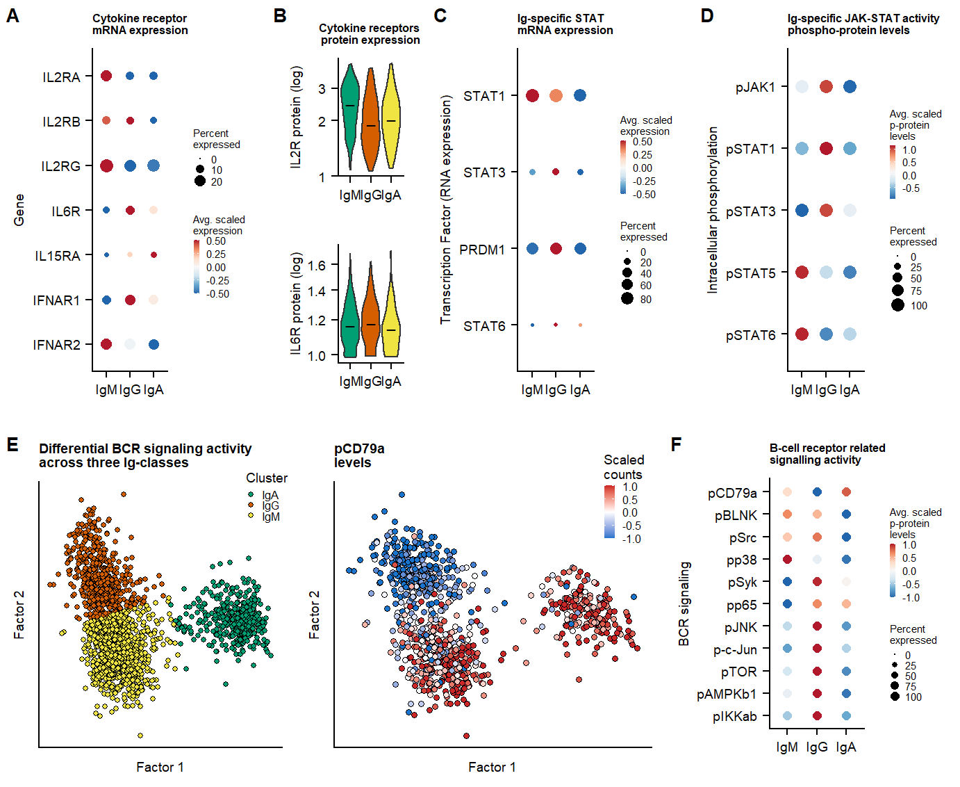

Differential geneexpression per Ig-class (suppl)

## RNA sign Differences

markers.OnevsAll <- FindAllMarkers(seu.live, assay = "SCT", logfc.threshold = 0.01, test.use = "wilcox", only.pos = T, verbose = T)
markers.OnevsAll <- filter(markers.OnevsAll, p_val <= 0.05)
markers.IgMvsAll <- filter(markers.OnevsAll, cluster == "IgM")
markers.IgAvsAll <- filter(markers.OnevsAll, cluster == "IgA")
markers.IgGvsAll <- filter(markers.OnevsAll, cluster == "IgG")

markers.IgAvsAll.list <- unique(replace(rownames(markers.IgAvsAll), rownames(markers.IgAvsAll)=="JCHAIN1", "JCHAIN"))
markers.OnevsAll.list <- unique(replace(rownames(markers.OnevsAll), rownames(markers.OnevsAll)=="JCHAIN1", "JCHAIN"))

p.dotplot.diff.genes.all <- DotPlot(seu.live,assay = "SCT", features =  rev(markers.OnevsAll.list), group.by =  "clusters_pcaIG_named", cols = "RdBu",dot.scale = 2,scale.min = 0, scale.max = 100, scale = T, scale.by = "size", col.min = -1, col.max = 1) +
  cowplot::theme_cowplot() + 
  coord_flip()+
  add.textsize +
  theme(legend.position = "right", legend.key.size = unit(2, 'mm'))

p.dotplot.diff.genes.IgM <- DotPlot(seu.live,assay = "SCT", features =  rev(rownames(markers.IgMvsAll)),split.by = "donor", cols = "RdBu",dot.scale = 2,scale.min = 0, scale.max = 100, scale = T, scale.by = "size", col.min = -1, col.max = 1) +
  cowplot::theme_cowplot() + 
  coord_flip()+
  add.textsize +
  theme(legend.position = "none", legend.key.size = unit(2, 'mm'))+
  labs(title="IgM versus others (88 genes)",x="Differential expressed genes (p-val < 0.05, logfc >= 0.01)", y = "") +
  scale_y_discrete(labels = c("D32 \n","D33 \nIgM", "D40","D32 \n","D33 \nIgG", "D40","D32 \n","D33 \nIgA", "D40"))

p.dotplot.diff.genes.IgA <- DotPlot(seu.live,assay = "SCT", features =  rev(markers.IgAvsAll.list),split.by = "donor", cols = "RdBu",dot.scale = 2,scale.min = 0, scale.max = 100, scale = T, scale.by = "size", col.min = -1, col.max = 1) +
  cowplot::theme_cowplot() + 
  coord_flip()+
  add.textsize +
  theme(legend.position = "none", legend.key.size = unit(2, 'mm'))+
  labs(title="IgA versus others (28 genes)",x="Differential expressed genes (p-val < 0.05, logfc >= 0.01)", y = "")+
  scale_y_discrete(labels = c("D32 \n","D33 \nIgM", "D40","D32 \n","D33 \nIgG", "D40","D32 \n","D33 \nIgA", "D40"))

p.dotplot.diff.genes.IgG <- DotPlot(seu.live,assay = "SCT", features =  rev(rownames(markers.IgGvsAll)),split.by = "donor", cols = "RdBu",dot.scale = 2,scale.min = 0, scale.max = 100, scale = T, scale.by = "size", col.min = -1, col.max = 1) +
  cowplot::theme_cowplot() + 
  coord_flip()+
  add.textsize +
  theme(legend.position = "right", legend.key.size = unit(2, 'mm'))+
  labs(title="IgG versus others (67 genes)",x="Differential expressed genes (p-val < 0.05, logfc >= 0.01)", y = "")+
  scale_y_discrete(labels = c("D32 \n","D33 \nIgM", "D40","D32 \n","D33 \nIgG", "D40","D32 \n","D33 \nIgA", "D40"))

p.suppl.diff.genes <- plot_grid(p.dotplot.diff.genes.IgM,p.dotplot.diff.genes.IgG, p.dotplot.diff.genes.IgA,ncol = 2, rel_widths = c(1,1.3), rel_heights = c(1,0.7), labels = panellabels[1:3], label_size = 10)


# ggsave(p.suppl.diff.genes, filename = "output/paper_figures/p.suppl.diff.genes.pdf", width = 183, height = 320, units = "mm",  dpi = 300, useDingbats = FALSE)
# ggsave(p.suppl.diff.genes, filename = "output/paper_figures/p.suppl.diff.genes.png", width = 183, height = 320, units = "mm",  dpi = 300)
p.suppl.diff.genes

Session information

sessionInfo()

R version 4.0.3 (2020-10-10)
Platform: x86_64-w64-mingw32/x64 (64-bit)
Running under: Windows 10 x64 (build 19044)

Matrix products: default

locale:
[1] LC_COLLATE=English_Netherlands.1252  LC_CTYPE=English_Netherlands.1252   
[3] LC_MONETARY=English_Netherlands.1252 LC_NUMERIC=C                        
[5] LC_TIME=English_Netherlands.1252    

attached base packages:
[1] parallel  stats4    stats     graphics  grDevices utils     datasets 
[8] methods   base     

other attached packages:
 [1] MOFA2_1.1.17           ggupset_0.3.0          RColorBrewer_1.1-2    
 [4] clusterProfiler_3.18.1 enrichplot_1.10.2      UCell_1.0.0           
 [7] data.table_1.14.2      scales_1.1.1           cowplot_1.1.1         
[10] ggthemes_4.2.4         kableExtra_1.3.4       knitr_1.36            
[13] org.Hs.eg.db_3.12.0    AnnotationDbi_1.52.0   IRanges_2.24.1        
[16] S4Vectors_0.28.1       Biobase_2.50.0         BiocGenerics_0.36.1   
[19] forcats_0.5.1          stringr_1.4.0          dplyr_1.0.7           
[22] purrr_0.3.4            readr_2.1.0            tidyr_1.1.4           
[25] tibble_3.1.5           ggplot2_3.3.5          tidyverse_1.3.1       
[28] Matrix_1.3-4           SeuratObject_4.0.2     Seurat_4.0.2          
[31] workflowr_1.6.2       

loaded via a namespace (and not attached):
  [1] utf8_1.2.2            reticulate_1.22       tidyselect_1.1.1     
  [4] RSQLite_2.2.8         htmlwidgets_1.5.4     BiocParallel_1.24.1  
  [7] grid_4.0.3            Rtsne_0.15            scatterpie_0.1.7     
 [10] munsell_0.5.0         codetools_0.2-16      ica_1.0-2            
 [13] future_1.23.0         miniUI_0.1.1.1        withr_2.5.0          
 [16] colorspace_2.0-2      GOSemSim_2.16.1       filelock_1.0.2       
 [19] highr_0.9             rstudioapi_0.13       ROCR_1.0-11          
 [22] tensor_1.5            DOSE_3.16.0           listenv_0.8.0        
 [25] labeling_0.4.2        MatrixGenerics_1.2.1  git2r_0.28.0         
 [28] polyclip_1.10-0       pheatmap_1.0.12       bit64_4.0.5          
 [31] farver_2.1.0          rhdf5_2.34.0          downloader_0.4       
 [34] rprojroot_2.0.2       basilisk_1.2.1        parallelly_1.29.0    
 [37] vctrs_0.3.8           generics_0.1.1        xfun_0.26            
 [40] R6_2.5.1              graphlayouts_0.7.2    rhdf5filters_1.2.1   
 [43] DelayedArray_0.16.3   fgsea_1.16.0          spatstat.utils_2.2-0 
 [46] cachem_1.0.6          assertthat_0.2.1      vroom_1.5.6          
 [49] promises_1.2.0.1      ggraph_2.0.5          gtable_0.3.0         
 [52] globals_0.14.0        goftest_1.2-2         tidygraph_1.2.0      
 [55] rlang_0.4.11          systemfonts_1.0.3     splines_4.0.3        
 [58] lazyeval_0.2.2        spatstat.geom_2.2-2   broom_0.7.10         
 [61] BiocManager_1.30.16   yaml_2.2.1            reshape2_1.4.4       
 [64] abind_1.4-5           modelr_0.1.8          backports_1.3.0      
 [67] httpuv_1.6.3          qvalue_2.22.0         tools_4.0.3          
 [70] ellipsis_0.3.2        spatstat.core_2.3-0   jquerylib_0.1.4      
 [73] ggridges_0.5.3        Rcpp_1.0.7            plyr_1.8.6           
 [76] basilisk.utils_1.2.2  rpart_4.1-15          deldir_1.0-2         
 [79] pbapply_1.5-0         viridis_0.6.2         zoo_1.8-9            
 [82] haven_2.4.3           ggrepel_0.9.1         cluster_2.1.0        
 [85] fs_1.5.0              magrittr_2.0.1        scattermore_0.7      
 [88] DO.db_2.9             lmtest_0.9-38         reprex_2.0.1         
 [91] RANN_2.6.1            whisker_0.4           fitdistrplus_1.1-6   
 [94] matrixStats_0.61.0    hms_1.1.1             patchwork_1.1.1      
 [97] mime_0.12             evaluate_0.14         xtable_1.8-4         
[100] readxl_1.3.1          gridExtra_2.3         compiler_4.0.3       
[103] shadowtext_0.0.9      KernSmooth_2.23-17    crayon_1.4.2         
[106] htmltools_0.5.2       ggfun_0.0.4           mgcv_1.8-33          
[109] later_1.3.0           tzdb_0.2.0            lubridate_1.8.0      
[112] DBI_1.1.1             corrplot_0.92         tweenr_1.0.2         
[115] dbplyr_2.1.1          rappdirs_0.3.3        MASS_7.3-53          
[118] cli_3.6.0             igraph_1.2.6          pkgconfig_2.0.3      
[121] rvcheck_0.2.1         plotly_4.10.0         spatstat.sparse_2.0-0
[124] xml2_1.3.2            svglite_2.0.0         bslib_0.3.1          
[127] webshot_0.5.2         rvest_1.0.2           yulab.utils_0.0.4    
[130] digest_0.6.28         sctransform_0.3.2     RcppAnnoy_0.0.19     
[133] spatstat.data_2.1-0   fastmatch_1.1-3       rmarkdown_2.11       
[136] cellranger_1.1.0      leiden_0.3.9          uwot_0.1.10          
[139] shiny_1.7.1           lifecycle_1.0.1       nlme_3.1-149         
[142] jsonlite_1.7.2        Rhdf5lib_1.12.1       limma_3.46.0         
[145] viridisLite_0.4.0     fansi_0.5.0           pillar_1.6.4         
[148] lattice_0.20-41       fastmap_1.1.0         httr_1.4.2           
[151] survival_3.2-7        GO.db_3.12.1          glue_1.4.2           
[154] png_0.1-7             bit_4.0.4             HDF5Array_1.18.1     
[157] ggforce_0.3.3         stringi_1.7.5         sass_0.4.0           
[160] blob_1.2.2            memoise_2.0.1         irlba_2.3.3          
[163] future.apply_1.8.1